Designing a Vector Database: Architecture, Filtered Search, and Multi-Tenancy
When I design a vector database like Pinecone, Milvus, Qdrant or Weaviate, the first surprise is how little of the hard work is the index itself. HNSW and IVF are well understood, and a single node running a good library can answer a nearest neighbor query over a few million vectors in a millisecond or two. The trouble starts when the corpus is a billion vectors spread across fifty thousand customers, every query carries a metadata filter, documents are being re-embedded and upserted all day, and the finance team wants to know why the bill grew faster than the data.
So the design problem is less "which ANN algorithm" and more a classic distributed storage problem with an unusual index in the middle: where the bytes live, how writes become searchable, how filters interact with approximate search, and how one tenant's traffic stays out of another's way. Those are the questions this post is about.
I walk through how I would build this system from scratch: scoping, requirements with capacity estimates, a high-level architecture, and then four deep-dives:
- Distributed architecture with storage-compute separation and serverless indexes
- Filtered ANN search that keeps recall when filters are selective
- Freshness: real-time upserts versus index rebuilds
- Multi-tenancy, isolation and cost
Scoping the Problem and Clarifying Assumptions
I am building a managed, multi-tenant vector database: a service that stores embeddings with metadata and answers "give me the k most similar items that also match this filter". It sits underneath RAG, semantic search, recommendations and deduplication, and does not care which one is calling.
What I'm including:
- Collections (I call them namespaces) holding vectors of a fixed dimension, each with a primary key and a JSON-like metadata payload
- Upsert, delete, fetch by id, and top-k similarity search with metadata filters
- Configurable consistency per query, from "eventually" up to "read your own writes"
- Thousands of tenants on shared infrastructure, with a path to dedicated capacity for large ones
- Usage metering for billing on storage, reads and writes
What I'm NOT building here:
- The embedding models. Callers send vectors.
- The RAG application layer: chunking, prompt assembly, permission sync from source systems. The enterprise RAG assistant design covers that side, including how ACLs get into the index in the first place.
- A full-text search engine. I support sparse vectors for hybrid search, but not analyzers, stemming or phrase queries.
Key assumptions:
- Dense vectors of 768 to 1,536 dimensions, float32 on the wire. I use 768 for the estimates.
- Cosine or inner-product similarity, with recall@10 of at least 0.95 against exact search as the default quality bar.
- Runs on a public cloud with an object store (S3-class), local NVMe on compute nodes, and a managed log or my own replicated log.
- The workload is skewed: a small share of namespaces receive most of the queries, and most namespaces are small and idle most of the day.
How this differs from a classic database: in a B-tree or LSM store, a lookup is exact and an update just changes a row. Here the index is approximate, so every choice is measured in recall as well as latency, the structures are expensive to build and hard to update in place, and the most common query shape, "similar AND matches a predicate", is the one approximate indexes handle worst. I recap the index algorithms in one line each and lean on Storage Engines and Indexes Compared for the internals: HNSW is a layered proximity graph walked greedily toward the query, and IVF clusters vectors around trained centroids and scans only the nearest clusters, optionally with product quantization to compress them.
Functional and Non-Functional Requirements
Functional Requirements
- Upsert a batch of
(id, vector, metadata)records into a namespace. Re-upserting an id replaces the old record. - Delete by id, by id list, or by metadata filter.
- Query for the top k nearest vectors with an optional filter, returning ids, scores and selected metadata.
- Fetch records by id.
- Consistency control: each query can ask for eventual, bounded-staleness or read-your-writes visibility.
- Namespace lifecycle: create, describe, resize, back up and drop a namespace, including fast hard-delete of all of a tenant's data.
Non-Functional Requirements
| Requirement | Target | Why |
|---|---|---|
| Query latency (warm namespace) | p50 under 20 ms, p99 under 100 ms for k = 10 | It sits inside RAG and search requests that have their own budgets |
| Query latency (cold namespace) | p99 under 1 to 2 s for the first query | Serverless tenants accept a cold start, not a timeout |
| Recall@10 | at least 0.95 by default, including filtered queries | Missing the right chunk breaks the answer upstream |
| Write visibility | under 1 to 2 s from ack to searchable | Users expect a newly added document to show up |
| Durability | no acknowledged write lost | Customers treat it as a system of record more often than they should |
| Availability | 99.9% for reads, 99.95% for writes | Writes can be logged even when search is degraded |
| Isolation | one tenant cannot push another's p99 past target | Shared fleet across thousands of tenants |
I track recall as an SLO next to latency. A faster query that quietly drops recall is a regression nobody notices until the RAG answers get worse.
Back-of-the-Envelope Capacity Estimation
These numbers are my planning assumptions, not measurements. The method matters more than the exact values: size the bytes per vector in each representation, then decide which representations must live in RAM.
Corpus:
- 50,000 namespaces, 1 billion vectors in total, heavily skewed (a few hundred namespaces over 10 million vectors, most under 100,000)
- 768 dimensions, plus about 500 bytes of metadata per record
float32 vectors:   1e9 x 768 x 4 bytes        = ~3.1 TB
int8 (scalar q.):  1e9 x 768 x 1 byte         = ~0.77 TB
PQ, 96 bytes/vec:  1e9 x 96 bytes             = ~0.1 TB
HNSW links, M=16:  1e9 x 32 links x 4 bytes   = ~0.13 TB (layer 0 only)
metadata:          1e9 x 500 bytes            = ~0.5 TB
Keeping everything in RAM at full precision, replicated, would be over 10 TB of memory. Full-precision vectors are needed only to re-rank a few hundred candidates per query, so they can live on NVMe or object storage. The compressed vectors and graph or centroids are what search walks, so only their hot part must be in RAM.
Hot set: if I assume about 20% of the data receives almost all queries, the hot in-memory footprint is roughly 0.2 x (0.77 TB int8 + 0.13 TB links) ≈ 180 GB, plus metadata indexes for filtering. That fits on a handful of large-memory nodes, so query nodes are sized by QPS, not memory, for the hot set.
Reads: 10,000 queries per second on average, 30,000 at peak. Suppose benchmarking shows one 32-core query node sustains about 2,000 filtered queries per second against hot segments within the p99 target. Peak then needs 30,000 / 2,000 = 15 nodes, and with 2 replicas per hot segment and 30% headroom, about 40 query nodes for the warm tier. Cold namespaces are served on demand from object storage by the same pool.
Writes: 2,000 upserts per second on average, 10,000 at peak, at about 3.6 KB each. That is 7 MB/s on average and 36 MB/s at peak into the log, about 170 million upserts and 600 GB of log per day. Modest for a log, but about 17% of the corpus rewritten daily, which is why deletes and compaction get their own deep-dive.
High-Level Architecture and Core Components
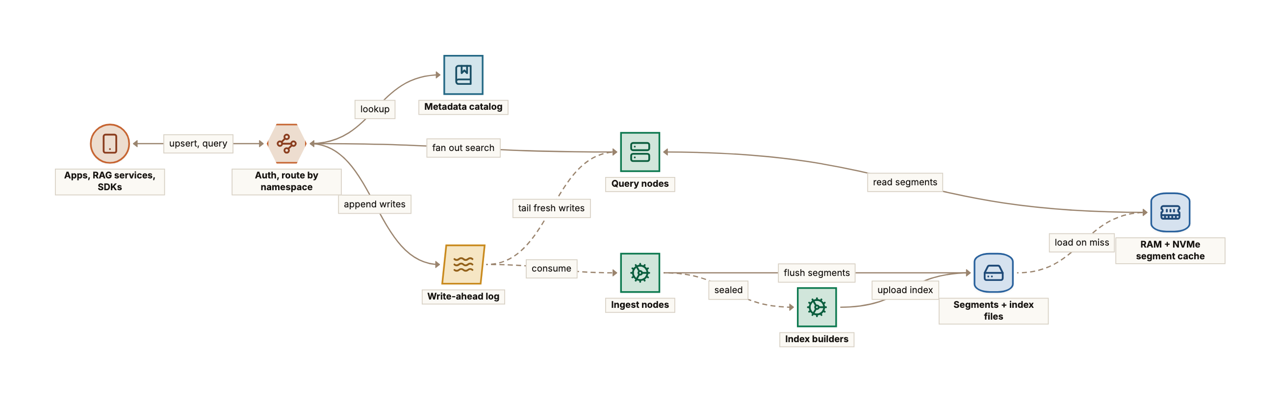
Component Walkthrough
API Gateway. Authenticates the API key, derives the tenant from it (never from the request body), validates dimensions, applies per-tenant rate limits, and looks up the namespace's shards and query nodes in the catalog.
Metadata catalog. The source of truth for namespaces, index settings, segments per shard, and segment-to-node assignments. Small, strongly consistent and read-heavy, so I keep it in a consensus-backed store (etcd or a small replicated SQL database) with a read cache in each gateway.
Write-ahead log (WAL). Every upsert and delete is appended to a partitioned, replicated log before it is acknowledged. The log, not any node's memory, is the durability point. Partitions are assigned by hash(namespace, shard), so one shard's writes are totally ordered.
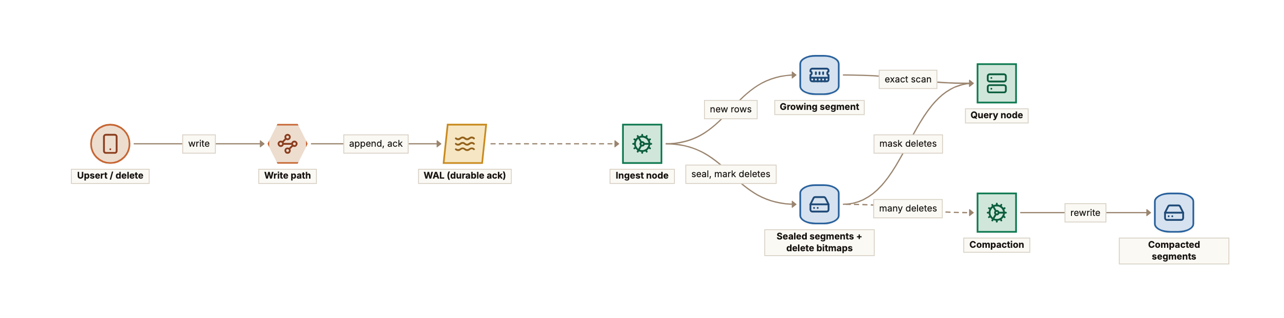
Ingest nodes. Consume log partitions, build growing segments in memory, and at a target size or age seal and flush them to object storage as immutable files: vectors, metadata columns and a bloom filter on ids.
Index builders. Build the ANN index for each sealed segment (HNSW for hot ones, IVF-PQ or a disk-oriented graph for large cold ones), plus metadata indexes, on their own autoscaled pool, never on query nodes.
Object storage. Holds every segment, index file and delete bitmap: the durable copy of all data. Compute nodes are caches in front of it.
Query nodes and coordinator. Query nodes are stateless. A coordinator assigns them segments with leases and reassigns on failure. They keep segments in a RAM and NVMe cache, return per-segment top-k lists, and tail the WAL so writes not yet sealed are searchable.
This follows the broad pattern of the published Milvus 2.x architecture (proxies, coordinators, data, index and query nodes over a log and object storage) and the storage-compute separation Pinecone has described for its serverless product. It is simply what falls out once object storage is the system of record.
Request Flow
Write:
- The client sends
POST /namespaces/docs-acme/upsertwith 200 records. - The gateway authenticates, validates and routes each record to its shard by hashing the id.
- The records are appended to that shard's WAL partition. Once replicated, the gateway returns the log position as a write token.
- Within a second or so, ingest and query nodes consume the entry and the records become searchable.
Query:
- The client sends a query vector,
top_k = 10, and a filter such as{"lang": "en", "year": {"$gte": 2024}}. - The gateway finds the namespace's shards and the query nodes holding their segments.
- Each query node plans the filter for each segment (deep-dive 2), searches it, and returns its local top k.
- The gateway merges the lists, optionally re-ranks the best few hundred candidates with full-precision vectors, and returns the top 10.
Scaling It Out
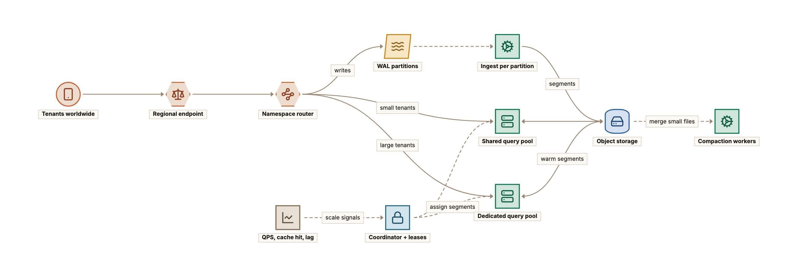
- Shards for writes, segments for reads. A namespace is split into a small number of shards for write ordering. Each shard holds many segments, and segments are the unit of placement, caching and indexing. A query node can hold segments from many namespaces.
- Replicate hot segments, not cold ones. Durability comes from object storage, so I replicate in compute only for throughput and fast failover. Hot segments get two or three query-node replicas. Cold ones get zero until queried.
- Separate pools. Large or latency-sensitive tenants get a dedicated query pool. Everyone else shares a pool. Index builders and compaction workers have their own pools, so a big rebuild never steals query CPU.
- Scale on the right signals. Query nodes on QPS, cache hit rate and p99; ingest on log lag. CPU alone misleads, because a node waiting on object storage looks idle.
- Regions. Each region is an independent deployment and a namespace has one home region. Cross-region read replicas copy sealed segments between buckets.
Deep-Dive: Distributed Architecture: Storage-Compute Separation and Serverless Indexes
Shared-Nothing vs Disaggregated
There are two basic ways to build this.
Shared-nothing, the classic search-cluster model: each node owns shards on local disk, with replicas for durability. Reads are always local, but storage and compute are coupled: more data means more nodes with CPU I may not need, rebalancing means copying shards, and every replica is a full copy on expensive storage.
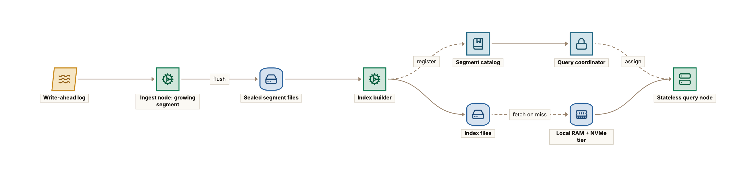
Disaggregated, the model I choose: object storage holds all data durably, and compute nodes are caches that can be added or replaced at will. A node failure loses nothing but warm cache. Once three-way SSD replication is counted, object storage is typically several times cheaper per stored GB. The price is a cache miss that costs tens of milliseconds. The rest of this deep-dive is about hiding that.
Segments Are the Unit of Everything
Each shard's data lives in immutable segments. I target about 1 million vectors per sealed segment (about 3 GB in float32, under 1 GB in int8): small enough to index in minutes and move quickly.
A sealed segment is a set of files plus a manifest in the catalog:
{
  "segment_id": "seg_7f3a",
  "namespace": "docs-acme",
  "shard": 3,
  "state": "sealed",
  "row_count": 1048576,
  "wal_range": [918223001, 919271576],
  "files": {
    "vectors_f32": "s3://vdb-prod/ns/docs-acme/seg_7f3a/vec.f32",
    "vectors_int8": "s3://vdb-prod/ns/docs-acme/seg_7f3a/vec.i8",
    "index": "s3://vdb-prod/ns/docs-acme/seg_7f3a/hnsw_m16.idx",
    "metadata": "s3://vdb-prod/ns/docs-acme/seg_7f3a/meta.parquet",
    "id_bloom": "s3://vdb-prod/ns/docs-acme/seg_7f3a/ids.bloom",
    "delete_bitmap": "s3://vdb-prod/ns/docs-acme/seg_7f3a/del.v12.roaring"
  },
  "index_params": { "type": "hnsw", "m": 16, "ef_construction": 200, "quant": "int8" }
}
Immutability keeps the design simple: any node can cache a segment without coordination and a cached copy is never stale. Updates become new data plus a versioned delete bitmap (deep-dive 3), and compaction replaces whole segments atomically in the catalog.
Tiered Caching on Query Nodes
Each query node has three tiers:
- RAM: the search structures for its assigned hot segments (graph links or IVF centroids, compressed vectors, metadata bitmaps).
- Local NVMe: full-precision vectors for re-ranking, and search structures for warm segments that do not fit in RAM. A disk-oriented graph index in the style of DiskANN works well here, because it is designed so that each search hop is one SSD read.
- Object storage: everything else.
Hot segments are pre-warmed before the coordinator routes traffic to a node; cold ones fill lazily. With range reads, a cold query fetches only the small routing structures (centroids or top graph layers) and then only the clusters or neighborhoods it needs, so the first query costs hundreds of milliseconds to low seconds rather than a multi-gigabyte download.
Query Fan-Out and Merge
A query touches every segment of the namespace, then merges: one or two for a small namespace, about 100 for a 100-million-vector one.
# Gateway-side scatter/gather with oversampling and full-precision re-rank
def search(namespace, q, k, flt, consistency):
    plan = catalog.segments_for(namespace)              # sealed + growing
    k_local = max(k, int(k * OVERSAMPLE))               # e.g. 2x to 4x
    futures = [node.search(seg, q, k_local, flt, consistency)
               for node, seg in plan.assignments()]
    candidates = heapq.nlargest(RERANK_POOL,
                                chain.from_iterable(f.result(timeout=0.08)
                                                    for f in futures),
                                key=lambda c: c.approx_score)
    exact = rerank_with_f32(candidates, q)              # NVMe or object store
    return exact[:k]
Three details matter in practice:
- Oversample per segment. Local search is approximate and int8 or PQ scores are noisy. Asking each segment for 2 to 4 times k and re-ranking at full precision recovers most of the lost recall cheaply.
- Tail latency is the max of many. I hedge to a second replica when a hot segment is slow, and a per-segment timeout returns partial results with a flag rather than failing the query.
- Prune. Per-segment min/max and value sets let the planner skip segments that cannot match a filter.
What "Serverless" Actually Means Here
For the tenant, serverless means no pods to size: they pay for GB-months, read units and write units, and idle namespaces scale to zero. For me, it falls out of the disaggregated design: an idle namespace costs only its object storage, the first query makes the coordinator assign its segments to a shared-pool node, and placement follows recent access, so popular namespaces climb into RAM and quiet ones fall out.
Failure modes. A herd of cold namespaces after a deploy or node loss can saturate object storage request rates. I rate-limit cache fills, prioritise segments by recent QPS, and keep a "last known hot set" in the catalog so a replacement node pre-warms the right segments before taking traffic.
What I would do first vs later. First: immutable segments on object storage, HNSW on int8 in RAM for hot segments, flat full-precision re-rank, scatter/gather with oversampling. Later: disk-oriented indexes for the warm tier, range-read cold starts, hedged requests, and access-driven placement.
Deep-Dive: Filtered ANN Search: Metadata Filters Without Losing Recall
Why Filters Are the Hard Part
Almost every real query has a filter: workspace, language, document type, date range, "in stock", and in RAG the user's permission groups. ANN indexes are built over the whole segment, not over "vectors where lang = en". The three basic strategies each fail predictably.
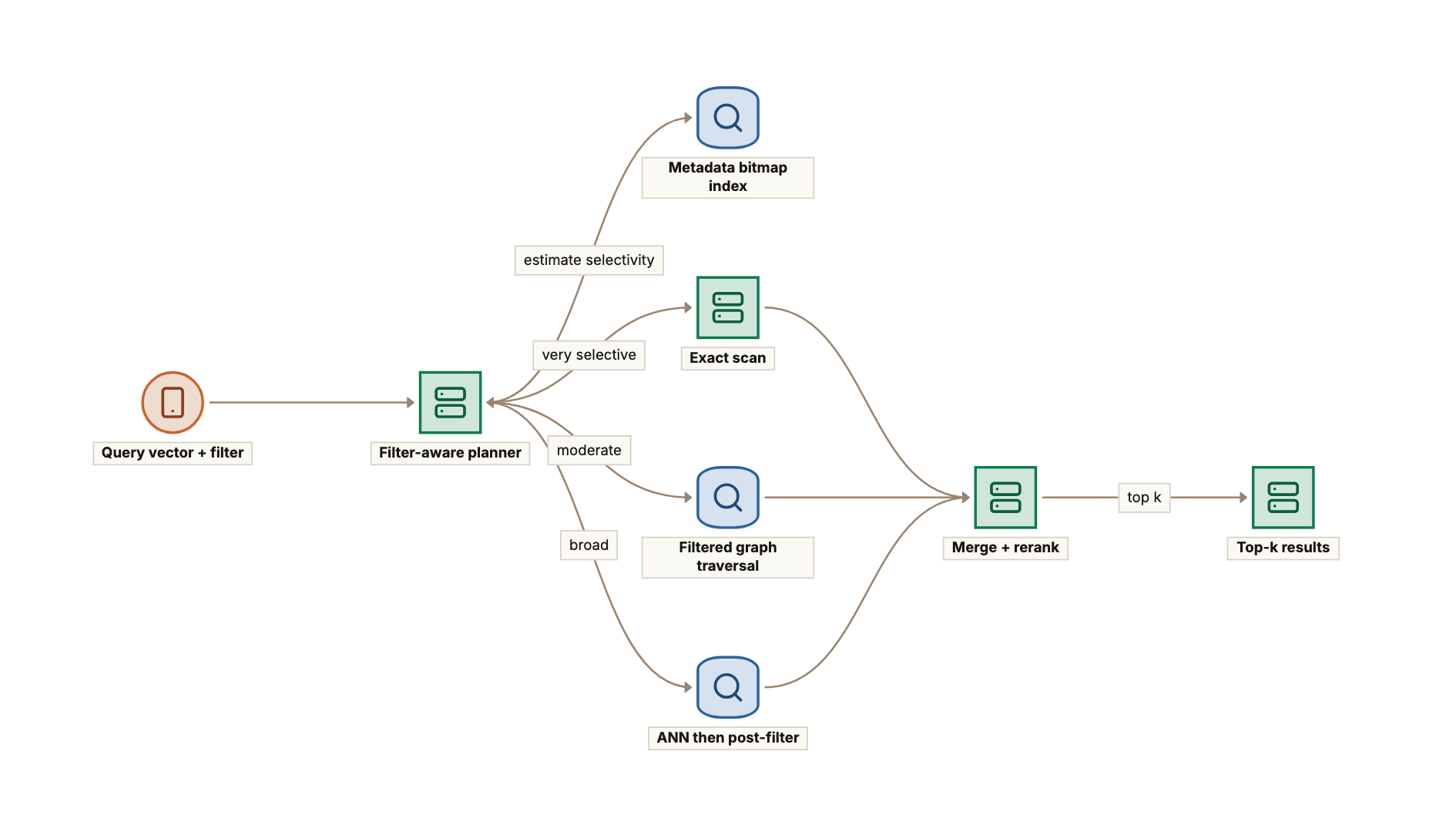
Post-filtering: run ANN for the top k' candidates, then drop those that fail the filter. Simple and fast when most vectors match. When only 1% match, the top 100 candidates contain about one match, so the query returns 1 result instead of 10. Raising k' until enough matches survive turns the query into a near scan.
Pre-filtering: compute the matching ids from a metadata index, then search only those. A small set means a fast exact scan with perfect recall. A large set makes the scan too slow.
In-filtering (filtered traversal): walk the graph or IVF lists as usual, but only admit matching vectors into results. Good at moderate selectivity. At low selectivity the matching nodes are sparse and poorly connected, the search wanders or gets stuck, and recall falls off a cliff.
Research systems attack exactly this cliff: ACORN builds a denser graph and expands neighbors-of-neighbors during filtered search, and Filtered-DiskANN builds label-aware graphs. I treat these as options for the index layer. The planner around them is what keeps recall predictable.
A Selectivity-Aware Planner
Each segment keeps metadata indexes: roaring bitmaps for low-cardinality fields (language, type, tags), sorted columns or a B-tree for numeric and date ranges, and an id-to-row map. Evaluating the filter against these indexes gives me the exact match count for the segment, cheaply. Then I choose a strategy per segment, not per query, because the same filter can match 80% of one segment and 0.1% of another.
def plan_segment(seg, flt, k):
    if flt is None:
        return Ann(seg, ef=EF_DEFAULT)
    matches = seg.meta_index.evaluate(flt)       # roaring bitmap
    n, total = len(matches), seg.row_count
    if n == 0:
        return Skip()
    if n <= EXACT_SCAN_MAX:                      # e.g. tens of thousands
        return ExactScan(seg, matches)           # perfect recall, cheap
    sel = n / total
    if sel >= BROAD_SELECTIVITY:                 # most rows match
        return AnnThenFilter(seg, matches, k_prime=int(k / sel * 1.5))
    # Moderate: filtered traversal, with ef scaled up as selectivity drops
    return FilteredAnn(seg, matches, ef=min(EF_MAX, int(EF_DEFAULT / sel)))
The thresholds are not universal. I tune them per index type on real query logs bucketed by selectivity and keep them in namespace config.
Partition Keys: Make the Common Filter Physical
If one field appears in nearly every query (a workspace id, a region), filtering on it is the wrong tool. Customers can declare it a partition key, and ingest writes different values into different segments. A query with workspace = 42 searches only that workspace's segments with no filter inside them, at unfiltered recall.
The trade-off is fragmentation: millions of tiny values would mean millions of tiny segments. I cap physical partitions and hash the long tail into shared bucket segments, where an exact scan separates them again.
Range and Multi-Field Filters
Combining fields is bitmap AND, OR and NOT; ranges come from sorted columns. The risky case is a filter broad on every field but selective in combination, such as lang = en AND type = contract AND year = 2019. Multiplying per-field estimates misjudges it, which is why I evaluate the full filter to an exact bitmap per segment. Over a million rows that costs little next to the vector search.
Measuring Filtered Recall
Average unfiltered recall hides the problem. A nightly job samples real queries with their filters, computes exact top k on a snapshot, and reports recall bucketed by selectivity (under 0.1%, 0.1 to 1%, 1 to 10%, over 10%). A planner or index change ships only if no bucket regresses.
Permission Filters
In RAG the filter often says "user is in one of these 300 groups", a large OR over a multi-valued field where in-filtering struggles. The database side is multi-valued bitmap indexes and the exact-scan path for very selective users. ACL sync and late-binding checks belong to the RAG design.
What I would do first vs later. First: bitmap metadata indexes, the three-way planner, partition keys, and selectivity-bucketed recall tests. Later: filter-aware graph construction for fields that are always filtered, learned thresholds, and hybrid dense plus sparse scoring with the same filter applied to both legs.
Deep-Dive: Freshness: Real-Time Upserts vs Index Rebuilds
The Tension
ANN indexes are built for read speed, not change. HNSW degrades under heavy churn and handles deletes awkwardly, IVF and PQ need trained centroids and codebooks, and large rebuilds take minutes to hours. Users still expect a new document to be searchable a second later, and a deleted one to vanish as fast.
My answer is the same as an LSM tree's: write to a small mutable structure, search it alongside large immutable ones, and merge in the background.
Writes: Log First, Then Growing Segments
- An upsert is appended to the shard's WAL. Once replicated, it is acknowledged with its log sequence number (LSN) as a write token.
- Ingest nodes and the query nodes serving that shard consume the log and add the record to a growing segment in memory.
- Growing segments are small, so I search them by exact scan (or a small incremental HNSW). A record is searchable as soon as it is consumed.
- On sealing, the segment is flushed and indexed. Query nodes serve the growing copy until the coordinator swaps in the indexed one.
Consistency Levels
Not every query needs the latest write. I expose four levels, similar to the consistency levels Milvus documents:
| Level | Guarantee | Cost |
|---|---|---|
| Eventual | Whatever the query node has consumed | None |
| Bounded staleness | Includes all writes older than N seconds | Query waits only if a node is far behind |
| Session | Includes writes made with this client's write token | Query waits until the node reaches that LSN |
| Strong | Includes every write acknowledged before the query started | Query waits until every involved node reaches the log head |
Session consistency is what most applications want: "after I upsert, my next query sees it". Query nodes report their consumed LSN per shard, and the gateway waits accordingly, with a timeout that returns results plus a "stale" flag. Strong is opt-in because it waits on the slowest node. Replication and Consistency Models covers the theory; the vector-specific point is that "consistent" means visible to search, which happens later than durable.
Upserts Are Deletes Plus Inserts
An upsert of an existing id must hide the old version. Each sealed segment's bloom filter on primary keys tells the ingest node which segments might hold the id; it confirms and records the row in that segment's versioned delete bitmap, which query nodes apply as a mask.
Masking is cheap but not free:
- Lost k. A top-10 with 3 deleted rows returns 7, so I oversample in proportion to the delete ratio.
- Graph quality. Deleted nodes still help navigation, but past some ratio the graph is mostly dead weight.
- Delete by filter is resolved at write time into row ids via the metadata indexes.
Compaction
Compaction workers rewrite segments to remove deleted rows and merge small segments. The policy is simple and tunable:
compaction:
  triggers:
    delete_ratio_above: 0.20        # rewrite when 20% of rows are dead
    small_segment_rows_below: 100000
    max_segments_per_shard: 512
  limits:
    max_concurrent_per_tenant: 2    # one tenant cannot hog the workers
    io_budget_mb_per_sec: 400       # per worker, protects object store limits
  output:
    target_rows: 1048576
    rebuild_index: true
    retain_old_segments_minutes: 30 # in-flight queries finish on old files
A compaction job drops masked rows, writes and indexes a new segment, then swaps it in atomically in the catalog: one transaction replaces the input ids with the output id. Old files are kept for a grace period so in-flight queries finish, and deletes that arrived during compaction are re-applied from the log using the manifest's LSN range.
Hard deletes. A delete is logically done when the bitmap is written, but the bytes remain in old files and the log. For data-subject deletion I force compaction of affected segments within a fixed window and bound log retention. Dropping a whole tenant is a prefix delete.
Full Index Rebuilds
Some changes cannot be done incrementally:
- A new embedding model. Old and new vectors are not comparable, so every vector must be regenerated.
- New index parameters (a different quantization, or HNSW to a disk graph).
- Drift. IVF centroids or PQ codebooks trained on last year's data fit poorly.
I build a new namespace version next to the old one: dual-write, backfill, shadow-read to compare recall and latency, then flip an alias atomically and keep the old version for a rollback window. Queries never see a half-built index. The cost is temporarily double storage and build compute.
What I would do first vs later. First: WAL-before-ack, growing segments with exact scan, delete bitmaps, delete-ratio compaction and session consistency. Later: incremental HNSW in growing segments, retraining quantizers in the background, and managed alias-based rebuilds for model migrations.
Deep-Dive: Multi-Tenancy, Isolation, and Cost
Three Ways to Place a Tenant
Tenant as a filter in one big index. Cheapest to run, worst on every other axis: each tenant is a selective filter that hits the recall cliff, a missing filter in application code leaks data across customers, and dropping a tenant means scattered deletes.
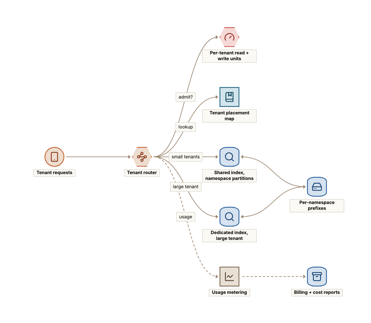
Namespace per tenant on shared infrastructure. Each tenant gets its own segments. Search runs unfiltered within the tenant, and dropping it is a prefix delete, while thousands of namespaces share query nodes and caches. This is my default.
Dedicated capacity. A large or regulated tenant gets its own query pool, and optionally its own builders and keys, at a much higher fixed cost.
Because data lives in object storage, moving a tenant to dedicated capacity is only a placement change: assign, pre-warm, flip the placement entry, release the shared copies.
placement_policy:
  default: shared
  promote_to_dedicated_when:
    sustained_qps_above: 500          # over 24 hours
    or_vectors_above: 50000000
    or_contract: provisioned
  shared_pool_limits_per_namespace:
    max_ram_cache_gb: 8
    max_concurrent_queries: 64
    max_index_build_jobs: 1
Noisy Neighbors
On shared query nodes, one tenant can hurt others in four ways, and each needs its own control:
- Query CPU. I meter queries in read units that track work done (vectors scored, bytes read), not requests, enforce per-tenant buckets at the gateway, and use weighted fair queuing on each query node. A k = 1,000 query on a 50-million-vector namespace costs far more than k = 10 on a small one.
- Cache. A one-off scan could evict everyone's hot segments, so each namespace has a cache quota and RAM admission requires repeated access.
- Write and compaction load. Bulk imports take a separate path (files straight to object storage, segments built offline), and each tenant's concurrent builds are capped.
- Object storage request rates. Prefixes get a hash component and cache fills are rate-limited.
Security Isolation
- Tenant identity comes from the credential, never a request field.
- Encryption at rest by default, and per-tenant data keys wrapped by a customer-controlled key on request. Revoking the key makes their segments unreadable.
- Per-namespace prefixes keep IAM policies, lifecycle rules and audits simple.
- Shared processes are the residual risk. A segment handle carries its namespace and the search API refuses mismatches, and CI tests for cross-tenant reads.
The Cost Model
My cost per tenant has three parts, and I try to make the price structure mirror them:
- Storage: object storage GB-months for vectors, indexes, metadata and retained old segments. Cheap per GB, and most of the bytes.
- Warm compute: query-node RAM and NVMe for hot segments and replicas. Expensive, and the main lever.
- Work: read and write units, plus build and compaction CPU.
For serverless, the margin depends on cache efficiency: read units served per GB of query-node RAM, the number I put on the dashboard per pool. The mistakes I watch for: float32 in RAM when int8 plus re-rank meets the recall bar, replicating cold segments in compute when object storage already provides durability, and old namespace versions lingering after a migration.
What I would do first vs later. First: namespace per tenant, read and write units with gateway buckets, per-namespace cache quotas, and per-namespace prefixes. Later: automatic promotion to dedicated pools, customer-managed keys, and cost reports per namespace that show customers which collections drive their bill.
Conclusion: Bringing It All Together
A vector database looks like a new kind of system, but most of its design is familiar distributed storage with one unusual constraint: the index is approximate and expensive to change, so every decision is judged by recall as well as latency and cost. Once that is clear, the architecture follows from a small number of choices.
If I had to summarise the design in four decisions:
- Make object storage the system of record and compute a cache. Immutable segments, a write-ahead log for durability, and stateless query nodes let storage and traffic scale independently, and give serverless and scale-to-zero almost for free.
- Plan filters per segment from exact bitmaps. Choose exact scan, filtered traversal or post-filtering by measured selectivity, make the most common filter a physical partition, and test recall per selectivity bucket.
- Treat freshness like an LSM tree. Log first, search growing segments by exact scan, mask deletes with bitmaps, compact in the background, and handle model migrations as versioned rebuilds behind an alias.
- Isolate tenants physically and meter work, not requests. Namespace per tenant on shared infrastructure by default, dedicated pools for the few who need them, and quotas on CPU, cache and builds so one tenant cannot spend another's latency budget.
Related reading: Storage Engines and Indexes Compared, Replication and Consistency Models, Designing an Enterprise RAG Assistant, and Block vs File vs Object Storage.