Storage Engines and Index Structures: B-Trees, LSM-Trees, Inverted Indexes, and Vector Indexes
Introduction
"Which database would you use?" is the question everyone prepares for. The follow-up that catches people is one level lower: "How does that database actually store the data, and why does that make your query fast?" Product names are labels. Underneath them sit a small number of storage engines and index structures, and those structures decide what is cheap, what is expensive, and what breaks first under load.
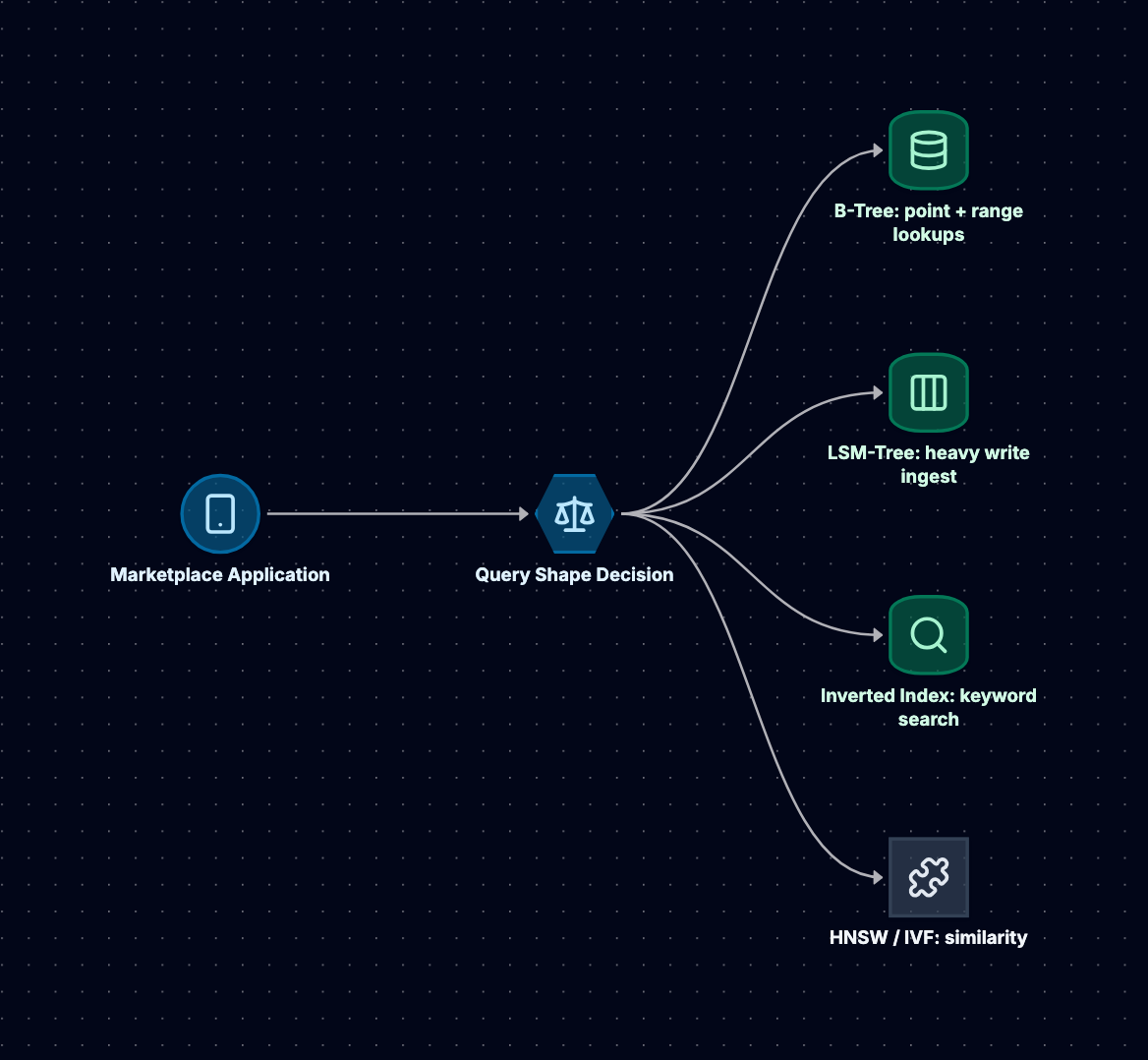
This post compares the four structures that cover almost every system design interview: the B-tree (PostgreSQL, MySQL InnoDB), the LSM-tree (Cassandra, RocksDB), the inverted index (Lucene, and therefore Elasticsearch and OpenSearch), and the vector index (HNSW and IVF, in pgvector or a dedicated vector database). For each: when to use it, how it works, a concrete example, how it scales, and how it fails.
We use one running example throughout: a marketplace with 10 million product listings. The marketplace needs four things:
- Fetch a listing by id and list a seller's listings by price (point and range lookups).
- Record product events (views, clicks, add-to-cart) at around 20,000 writes per second.
- Let shoppers search "waterproof hiking boots" and get relevant results (keyword search).
- Show "similar items" based on 768-dimension embeddings of each listing (semantic similarity).
Each of those is a different query shape, and each maps naturally to a different engine.
Why the Engine Matters More Than the Brand
Two databases with very different marketing can share an engine, and two databases with similar marketing can behave in opposite ways. CockroachDB and YugabyteDB speak SQL but store data in LSM-based key-value engines (Pebble and a RocksDB fork, respectively), so they inherit LSM write behavior, not PostgreSQL's heap behavior. MongoDB's WiredTiger engine is B-tree based by default. Elasticsearch is a distributed coordination layer over Lucene, so its refresh, merge, and deletion behavior is Lucene's. PostgreSQL with pgvector and a dedicated vector database may run the same HNSW algorithm with different operational trade-offs.
So the strong answer to "why Cassandra for the event stream?" is not "because Cassandra scales". It is: "The workload is append-heavy and read by key plus time range; an LSM-tree turns random writes into sequential ones, and Cassandra partitions it across nodes by key." Every engine trades among three costs:
- Read amplification: how much work (pages, files, I/Os) a single lookup costs.
- Write amplification: how many bytes the engine writes to disk for each byte the application writes.
- Space amplification: how much disk the engine uses relative to the live data.
The RUM conjecture (Athanassoulis and others, 2016) states it formally: an access method can optimize two of read, update, and memory overhead, not all three. B-trees favor reads, LSM-trees favor writes, and inverted and vector indexes accept expensive, batched writes to make one query shape fast.
B-Trees: PostgreSQL and InnoDB
When to Use It
A B-tree finds a key (or the first key above it) in a small, predictable number of page reads, then scans forward in sorted order. That covers equality, ranges, ORDER BY, composite-key prefixes, and uniqueness. Use it when reads matter more than raw write throughput and rows are updated transactionally. "Get listing 8812734" and "the 20 cheapest active listings for seller 42" are B-tree queries.
How It Works Internally
Both engines use B+trees of fixed-size pages: 8 KB in PostgreSQL, 16 KB by default in InnoDB. Internal pages hold separator keys and child pointers; leaf pages hold entries and link to siblings for range scans.
Fan-out keeps the tree shallow. An 8 KB page holds a few hundred small entries; at a fan-out of 300, three levels address 27 million entries. Our 10 million listings fit in depth three or four, with upper levels cached, so a point lookup costs one or two disk reads.
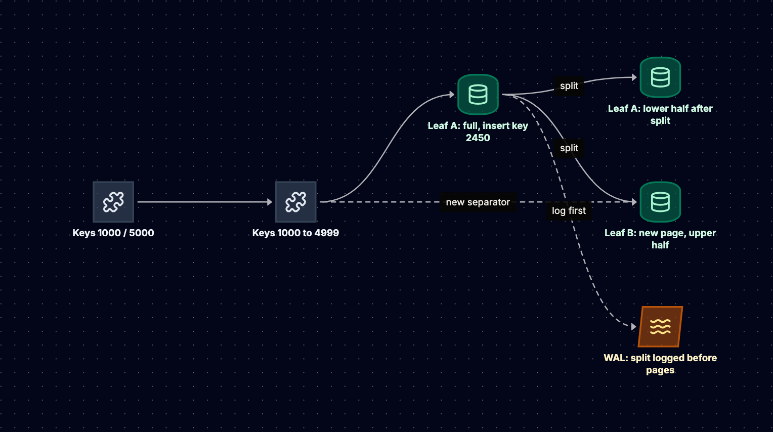
Page splits. An insert into a full leaf allocates a new page, moves about half the entries there, and adds a separator to the parent, which can split in turn; a root split grows the tree a level. Splits write several pages for one insert and leave pages half full.
Both engines special-case ever-increasing keys: PostgreSQL fills the rightmost leaf to its fill factor instead of splitting 50/50, and InnoDB detects sequential inserts similarly. Random keys (UUIDv4, hashes) get no help: splits happen everywhere, pages settle partly empty, and the hot working set becomes the whole index.
Fill factor is how full the engine packs a page when it has a choice. PostgreSQL B-tree indexes default to 90 and tables to 100; a lower table fill factor leaves room for updated row versions (see MVCC below). InnoDB's innodb_fill_factor applies to sorted index builds, and pages below MERGE_THRESHOLD (50 percent by default) are merged with a neighbor after deletes.
Write-ahead log. A split touches several pages, and a crash midway would corrupt the tree. So changes go first to a sequential log, flushed on commit, before pages are written back: the WAL in PostgreSQL, the redo log in InnoDB. Recovery replays it. PostgreSQL also logs a full page image on the first change to a page after each checkpoint (full_page_writes), an often overlooked source of WAL volume.
MVCC: where PostgreSQL and InnoDB really differ. Both give readers a snapshot without blocking writers, but they store old versions in different places.
- PostgreSQL: heap plus secondary indexes. Rows live in an unordered heap, and every index (primary key included) points to a physical tuple location (TID). An
UPDATEwrites a new tuple version and leaves the old one forVACUUM. Normally every index then gets a new entry, even on unchanged columns. A HOT update (heap-only tuple) avoids that when no indexed column changed and the new version fits on the same page, which is why a table fill factor of 80 to 90 helps update-heavy tables. - InnoDB: clustered index plus undo log. The table is the primary key B-tree: clustered index leaves hold full rows in key order. Secondary entries store the primary key value, so a secondary lookup is two traversals. Updates happen in place, the previous version goes to the undo log for older snapshots, and a purge thread cleans up later.
Consequences: in PostgreSQL, many indexes plus non-HOT updates means index write amplification and bloat, so autovacuum must stay healthy. In InnoDB, the primary key is a physical layout decision: a random UUID key means random inserts into the table itself, copied into every secondary index. Long-running transactions hurt both, holding back VACUUM or undo purge.
Example: The Listings Table
-- PostgreSQL: listings with room for HOT updates on the heap
CREATE TABLE listings (
  listing_id   BIGINT GENERATED ALWAYS AS IDENTITY PRIMARY KEY,
  seller_id    BIGINT       NOT NULL,
  title        TEXT         NOT NULL,
  price_cents  INT          NOT NULL,
  status       TEXT         NOT NULL,
  view_count   BIGINT       NOT NULL DEFAULT 0,   -- frequently updated, not indexed
  updated_at   TIMESTAMPTZ  NOT NULL DEFAULT now()
) WITH (fillfactor = 85);

-- Composite B-tree: equality on seller_id, range/sort on price
CREATE INDEX idx_listings_seller_price
  ON listings (seller_id, price_cents)
  WHERE status = 'active';

-- Served by one index range scan, already sorted
SELECT listing_id, title, price_cents
FROM listings
WHERE seller_id = 42 AND status = 'active'
ORDER BY price_cents
LIMIT 20;

-- Check whether updates are staying HOT
SELECT n_tup_upd, n_tup_hot_upd
FROM pg_stat_user_tables WHERE relname = 'listings';
-- MySQL InnoDB: the primary key is the physical row order
CREATE TABLE listings (
  listing_id   BIGINT UNSIGNED NOT NULL AUTO_INCREMENT,
  seller_id    BIGINT UNSIGNED NOT NULL,
  title        VARCHAR(300)    NOT NULL,
  price_cents  INT             NOT NULL,
  status       VARCHAR(16)     NOT NULL,
  PRIMARY KEY (listing_id),                       -- sequential: appends to the right edge
  KEY idx_seller_price (seller_id, price_cents)   -- entries carry listing_id implicitly
) ENGINE=InnoDB;
Leaving view_count unindexed keeps its updates HOT. Better still, do not update a row per view at all; that is what the event stream in the next section is for.
Scaling
Scale vertically first (more RAM keeps more of the tree cached), add read replicas fed by the WAL or binlog, then partition and shard by a key such as seller_id. The engine-level ceiling is random I/O: once the index outgrows memory, each random insert may read a page from disk before modifying it.
Failure Modes and Anti-Patterns
- Random primary keys in InnoDB. UUIDv4 splits pages across the clustered index and inflates secondary indexes. Prefer sequential ids or time-ordered ones such as UUIDv7.
- Too many indexes on update-heavy PostgreSQL tables. Every non-HOT update writes every index. Audit with
pg_stat_user_indexes. - Starved autovacuum. Bloat accumulates; a long-running transaction or abandoned replication slot is the usual culprit.
- Wrong composite column order. Equality columns first, then the range or sort column.
- Text search on a B-tree.
LIKE '%boots%'cannot use one. That is an inverted index's job.
LSM-Trees: Cassandra and RocksDB
When to Use It
The log-structured merge tree buffers writes in memory and writes them out as large, sorted, immutable files, turning random writes into sequential ones. Use it when writes dominate, data is mostly appended, and reads are by key or short key range. Our 20,000 events per second (about 1.7 billion per day, read as "events for listing X in the last hour") is the textbook case.
Cassandra is a distributed database with an LSM-tree on each node. RocksDB is an embeddable LSM library (forked from LevelDB) used inside systems such as Kafka Streams state stores and TiKV.
How It Works Internally
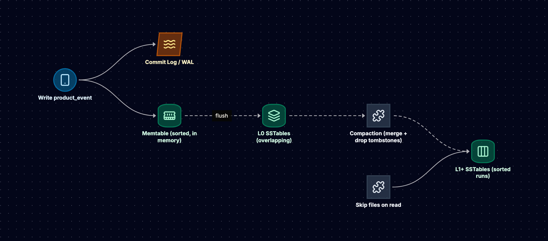
Write path. A write is appended to a commit log (Cassandra) or WAL (RocksDB), inserted into the in-memory sorted memtable, and acknowledged. No data page is read or modified. When the memtable fills (RocksDB's write_buffer_size defaults to 64 MB), it is frozen and flushed as an SSTable: an immutable file of sorted key-value pairs with a block index and usually a bloom filter (on by default in Cassandra; in RocksDB you enable it with filter_policy, for example a 10 bits-per-key bloom filter).
Read path. A point read checks the memtables, then SSTables: RocksDB goes newest to oldest and stops at the first match, while Cassandra merges row fragments from every SSTable that may hold the partition, reconciling cells by timestamp. Bloom filters keep this cheap: each SSTable's filter answers "definitely not here" or "possibly here", and at about 10 bits per key the false positive rate is roughly 1 percent (Cassandra exposes this as bloom_filter_fp_chance). Block indexes and a block cache handle the rest. Range scans get no bloom filter help and must merge iterators across overlapping files.
Updates and deletes. An update is a newer write of the same key; the newest wins at read time. A delete writes a tombstone marker. Shadowed versions and tombstones stay on disk until compaction.
Compaction merges SSTables, keeps the newest version of each key, and drops shadowed data and (eventually) tombstones. The strategy is the key LSM tuning decision:
- Size-tiered (Cassandra's long-standing default, STCS): merge several similar-sized SSTables (four by default) into one bigger file. Low write amplification, but a key can live in many overlapping files, and big compactions temporarily need room for input and output, so operators keep lots of disk free.
- Leveled (RocksDB's default, Cassandra's LCS): each level is typically 10 times the previous, and files within a level (L1 and above) do not overlap, so a point read touches at most one file per level and space overhead stays near 10 percent. The cost is write amplification: each level transition rewrites overlapping files, which can total tens of bytes written per byte ingested.
- Time-window (Cassandra's TWCS): for TTL'd time-series, group SSTables by time window and drop whole windows on expiry.
Cassandra 5.0 added the Unified Compaction Strategy (UCS), which can be tuned to behave tiered or leveled; check your version's default.
Example: The Product Events Table
-- Cassandra CQL: one partition per listing per day, newest first
CREATE TABLE product_events (
  listing_id  bigint,
  day         date,
  event_ts    timeuuid,
  event_type  text,
  user_id     bigint,
  PRIMARY KEY ((listing_id, day), event_ts)
) WITH CLUSTERING ORDER BY (event_ts DESC)
  AND compaction = {
    'class': 'TimeWindowCompactionStrategy',
    'compaction_window_unit': 'DAYS',
    'compaction_window_size': 1
  }
  AND default_time_to_live = 2592000;   -- 30 days

-- A single-partition slice: memtable plus a few SSTables in the same window
SELECT event_type, user_id FROM product_events
WHERE listing_id = 8812734 AND day = '2026-10-05'
LIMIT 100;
The (listing_id, day) key bounds partition size, and TWCS plus a TTL drops expired data as whole files. In RocksDB the same knobs look like this:
write_buffer_size = 64MB                  # memtable size before flush
max_write_buffer_number = 2               # memtables held before stalling writes
level0_file_num_compaction_trigger = 4    # L0 files before compaction into L1
max_bytes_for_level_multiplier = 10       # each level 10x the previous
compaction_style = kCompactionStyleLevel  # leveled (default) vs universal (tiered)
Scaling
Per node, ingest is bounded by compaction. When it falls behind, RocksDB slows and then stalls writes (on L0 file count and pending compaction bytes), which shows up as latency spikes. Across nodes, Cassandra hashes partition keys onto a token ring with (commonly) three replicas, so throughput scales near linearly if keys spread evenly.
Back-of-envelope: 20,000 writes per second at 200 bytes is 4 MB per second, about 345 GB per day raw. At replication factor 3 that is roughly 1 TB per day, before compaction multiplies physical writes. That is why compaction strategy is not a detail.
Failure Modes and Anti-Patterns
- Tombstone buildup. Reads scan past every tombstone in a partition. Cassandra warns at 1,000 per query and fails at 100,000 by default. Queue-like tables (insert, consume, delete) are the classic trap.
- Zombie data. Tombstones are kept for
gc_grace_seconds(10 days by default). A replica down longer than that, without repair, can resurrect deleted rows. - Size-tiered for read-heavy, overwrite-heavy tables. Reads touch many files; use leveled.
- Unbounded partitions. Bucket by time.
- Treating it as a query engine. Filtering on non-key columns means scans or costly distributed secondary indexes.
Inverted Indexes: Elasticsearch and Lucene
When to Use It
An inverted index maps each term to every document containing it. Use it for full-text search, text plus facets, log search, and autocomplete. "waterproof hiking boots" should match "Women's Hiking Boot, Waterproof Leather", which needs tokenizing, lowercasing, stemming, and relevance ranking. LIKE can do none of that.
How It Works Internally
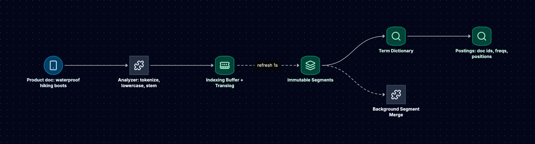
Analysis. Each text field passes through an analyzer: a tokenizer, then filters for lowercasing, stop words, stemming, or synonyms. Queries use the same analyzer, so "Boots" matches "boot".
Term dictionary and postings. Per field, Lucene keeps a sorted term dictionary (indexed by a compact finite state transducer). Each term points to a postings list: sorted document ids, usually with term frequencies, optionally positions (for phrases). Postings are delta-encoded and block-compressed. A three-word query looks up three terms and intersects or unions their lists, using skip data to jump ahead. Separately, column-oriented doc values serve sorting and aggregations.
Ranking with BM25 (the default since Lucene 6 and Elasticsearch 5.0). A document scores higher for a term when the term appears more often in it, with diminishing returns controlled by k1 (default 1.2); when the term is rare in the corpus (inverse document frequency); and when the field is short relative to average, controlled by b (default 0.75). Scores sum across terms. IDF is per shard by default, so uneven shards can rank slightly differently.
Segments, refresh, and merges. A Lucene index is a set of immutable segments, the LSM idea applied to search:
- New documents enter an in-memory buffer and, in Elasticsearch, a translog for durability.
- A refresh (every 1 second by default) turns the buffer into a searchable segment. Hence near real-time: durable on write, searchable after refresh. Since Elasticsearch 7.0, if
refresh_intervalis not set explicitly, shards idle for searches (30 seconds by default) skip scheduled refreshes; setting it, even to "1s", disables that optimization. - A flush is a Lucene commit, after which the translog can be trimmed.
- Deletes mark documents in a per-segment bitmap; an update is a delete plus an add.
- Background merges combine similar-sized segments and purge deleted documents, much like size-tiered compaction.
Example: Searching Listings
PUT /listings
{
  "settings": {
    "number_of_shards": 3,
    "number_of_replicas": 1,
    "refresh_interval": "1s"
  },
  "mappings": {
    "properties": {
      "title":       { "type": "text", "analyzer": "english" },
      "description": { "type": "text", "analyzer": "english" },
      "brand":       { "type": "keyword" },
      "price_cents": { "type": "integer" },
      "status":      { "type": "keyword" }
    }
  }
}

GET /listings/_search
{
  "query": {
    "bool": {
      "must":   { "multi_match": { "query": "waterproof hiking boots",
                                   "fields": ["title^3", "description"] } },
      "filter": [ { "term":  { "status": "active" } },
                  { "range": { "price_cents": { "lte": 15000 } } } ]
    }
  },
  "aggs": { "by_brand": { "terms": { "field": "brand" } } }
}
must is BM25-scored with titles boosted; filter clauses do not score and are cacheable; the brand facet reads doc values. PostgreSQL remains the system of record, feeding the index through CDC or an outbox, so it can always be rebuilt.
Scaling
An index splits into primary shards (each a Lucene index) plus replicas. A search fans out to every shard and merges, so latency follows the slowest shard. Primary shard count is fixed at creation (changeable via split, shrink, or reindex); the default is one since Elasticsearch 7.0. Time-based data uses an index per period behind an alias, so retention is deleting whole indexes. For backfills, use the bulk API and a longer (or disabled) refresh_interval.
Failure Modes and Anti-Patterns
- Search index as system of record. Mapping changes often need a reindex; keep truth elsewhere.
- Refreshing per write. Tiny segments and heavy merging.
- Mapping explosion. Dynamic mapping on arbitrary JSON bloats cluster state; use explicit mappings or
flattened. - Deep pagination.
max_result_windowdefaults to 10,000; usesearch_after. - Over-sharding. Many small shards waste memory and coordination.
- Hot counters in documents. Each update re-indexes the whole document; keep
view_countout.
Vector Indexes: HNSW, IVF, and pgvector vs Dedicated Vector Databases
When to Use It
A vector index finds the stored vectors closest to a query vector under cosine, L2, or inner product distance. The vectors are model embeddings, so close means semantically similar. Use it for semantic search, similar items, recommendations, deduplication, and LLM retrieval. Our "similar items" finds the "trail shoe, water-resistant" that shares no keywords with "hiking boots".
Exact search over 10 million 768-dimension vectors is about 7.7 billion multiply-adds per query: fine offline, too costly per page view. Indexes do approximate nearest neighbor (ANN) search, skipping most vectors and occasionally missing a true neighbor. Quality is measured as recall@k, the fraction of the true top k returned.
How It Works Internally
HNSW (Hierarchical Navigable Small World) is a multi-layer proximity graph (Malkov and Yashunin, 2016). Every vector is a node in layer 0, linked to near neighbors; each node is also randomly assigned a top layer with exponentially decreasing probability, so upper layers are sparse express lanes. Search enters at the top, greedily moves toward the query, descends when it cannot improve, and at layer 0 runs a beam search keeping ef_search candidates.
M: max links per node per layer (hnswlib and pgvector allow twice that on layer 0). Higher means better recall, more memory, slower builds.ef_construction: candidate list size during insert. Higher means a better graph and slower builds.ef_search: candidate list size at query time, the main runtime dial for recall versus latency. It must be at least k.
HNSW has strong recall and latency, incremental inserts, and no training step. It costs memory (the graph should stay in RAM), slow large builds, and awkward deletes.

IVF (inverted file index) clusters instead. Training runs k-means to produce lists centroids, and each vector joins its nearest centroid's list. A query compares against centroids and scans only the closest probes lists: 1,000 lists and 10 probes scans about 1 percent of the data. IVF builds faster and uses less memory than HNSW but usually has lower recall at equal speed, and centroids must be trained on representative data.
Recall versus latency. Raising ef_search or probes raises recall with diminishing returns and costs proportionally more work. Tune by measuring recall against exact search on real queries.
Quantization. Raw float32 for our listings is 10 million times 768 times 4 bytes, about 30.7 GB before the graph. Scalar quantization stores int8 (4x smaller) or float16 (2x) with small recall loss. Product quantization replaces sub-vectors with codebook ids for much higher compression and more loss. Binary quantization (32x) is a coarse first pass. The common pattern: fetch a few hundred candidates from a compressed index, then re-rank with full-precision distances.
Filtering. "Similar, active, under $150": post-filtering can return far fewer than k results when the filter is selective, and pre-filtering can degrade into a scan. Filtered search quality is a key differentiator between vector engines.
Example: pgvector on the Listings Table
CREATE EXTENSION IF NOT EXISTS vector;

ALTER TABLE listings ADD COLUMN embedding vector(768);

-- HNSW index (pgvector 0.5.0+); defaults are m = 16, ef_construction = 64
CREATE INDEX idx_listings_embedding
  ON listings USING hnsw (embedding vector_cosine_ops)
  WITH (m = 16, ef_construction = 64);

-- Query-time recall/latency dial (default 40)
SET hnsw.ef_search = 100;

-- pgvector 0.8.0+: keep scanning the index when filters remove too many rows
SET hnsw.iterative_scan = relaxed_order;

SELECT listing_id, title
FROM listings
WHERE status = 'active' AND price_cents <= 15000
ORDER BY embedding <=> $1      -- cosine distance to the query embedding
LIMIT 10;

-- Alternative: IVFFlat. Build after loading data; probes defaults to 1
-- CREATE INDEX ON listings USING ivfflat (embedding vector_cosine_ops) WITH (lists = 3000);
-- SET ivfflat.probes = 50;
pgvector's docs suggest IVFFlat lists of rows divided by 1,000 up to a million rows, the square root of rows beyond, and probes near the square root of lists: about 3,000 lists and 50 probes for us, as a starting point. The halfvec type and HNSW/IVFFlat indexing of PostgreSQL bit vectors (for binary quantization) arrived in pgvector 0.7.0.
pgvector vs a Dedicated Vector Database
pgvector is enough when the index fits in memory on one PostgreSQL node (millions to low tens of millions of vectors, depending on dimensions and hardware), you want deletes and updates to be transactionally consistent with similarity results, queries mix vectors with SQL filters and joins, and the team would rather not run and sync a second store.
A dedicated vector database (Milvus, Qdrant, Weaviate, Pinecone, or vector search in OpenSearch and Elasticsearch) earns its place when you need hundreds of millions of vectors sharded across nodes, high vector QPS isolated from OLTP traffic, stronger filtered search, quantization, disk-based indexes, multi-tenancy or hybrid ranking, or the ability to rebuild a re-embedded index on separate infrastructure and swap it in. The price is a second system kept in sync by CDC or an outbox, with eventual consistency.
Scaling
Memory is raw vectors plus links: at M = 16, up to 32 neighbor ids per node on layer 0 is about 128 bytes with 4-byte ids (hnswlib) or about 192 bytes with pgvector's 6-byte tuple ids, roughly 1.3 to 1.9 GB for 10 million vectors before upper layers and page overhead. Scale out by sharding and merging per-shard top k, like a search index; quantize to stay in memory.
Failure Modes and Anti-Patterns
- Never measuring recall. You cannot tell what a latency gain cost.
- Naive post-filtering. Selective filters return three results instead of ten; use iterative scans, partial indexes, or filter-aware engines.
- Mixing embedding models. Vectors from different models are not comparable; re-embed and rebuild.
- IVF built on an empty table. Centroids miss the real distribution.
- Graph on disk. HNSW collapses when every hop is a disk read.
- Vectors only. Embeddings are weak on SKUs and model numbers; hybrid with BM25 often wins.
Read, Write, and Space Amplification
The three amplification factors give a single vocabulary for every engine above.
B-tree. Low read amplification (one or two disk reads per lookup). Write amplification comes from page-granular writes: one 100-byte change dirties an 8 KB or 16 KB page plus WAL, and possibly a full page image, a worst case well over 100x that batching reduces. Space amplification comes from partly full pages and, in PostgreSQL, dead tuples.
LSM-tree. Write amplification is low for size-tiered and higher for leveled (tens of times is possible). Point reads cost more than a B-tree on cache misses, softened by bloom filters; range scans merge many files. Space is low for leveled, high for size-tiered, plus tombstones until compaction.
Inverted index. Segments are merged repeatedly, like tiered LSM, and updates re-index whole documents. Term reads scale with postings length and fan out to every shard.
Vector index. Each HNSW insert runs an ef_construction search and rewires neighbors. Read cost is set by ef_search or probes and trades against recall. Space is dominated by the vectors, hence quantization.
Say which amplification you accept and why the workload tolerates it.
Head-to-Head Comparison
| Dimension | B-Tree (PostgreSQL, InnoDB) | LSM-Tree (Cassandra, RocksDB) | Inverted Index (Lucene, Elasticsearch) | Vector Index (HNSW, IVF) |
|---|---|---|---|---|
| Best query shape | Point lookup, range scan, sorted order | Write-heavy key and key-range access | Full-text and filtered keyword search | Nearest neighbor by embedding |
| Write pattern | In-place page updates plus WAL | Append to log and memtable, flush, compact | Buffer, refresh into segments, merge | Per-vector graph insert or list assignment |
| Point read cost | Very low (shallow tree, cached internals) | Low with bloom filters, more files to check | Not its purpose | Not its purpose |
| Range scan | Excellent (sorted, linked leaves) | Good, merges iterators across files | Not its purpose | Not applicable |
| Write amplification | Moderate (page-sized writes, full page images) | Low (tiered) to high (leveled) | Moderate to high (repeated merges) | High per insert (graph search) |
| Space amplification | Moderate (fill factor, dead tuples) | Low (leveled) to high (tiered) | Moderate (postings, doc values, deleted docs) | High raw, reduced by quantization |
| Updates and deletes | In place (InnoDB) or new version (PostgreSQL) | New version or tombstone, resolved in compaction | Delete marker plus full re-index | Awkward; marked and cleaned later |
| Freshness | Immediate on commit | Immediate | Near real-time (default 1s refresh) | Immediate in pgvector; varies by engine |
| Exact or approximate | Exact | Exact | Exact matching, relevance-ranked | Approximate (tunable recall) |
| Main tuning knobs | Fill factor, indexes, VACUUM, PK choice | Compaction strategy, memtable size, bloom filters | Analyzers, refresh interval, shard count | M, ef_construction, ef_search, lists, probes, quantization |
| Typical role | System of record | High-volume event and key-value storage | Derived search view | Derived similarity view (or in-database with pgvector) |
Two rows matter most in an interview. Write pattern explains throughput: in-place updates force random I/O, while append-and-merge designs turn it into sequential I/O and pay later in compaction. Typical role explains architecture: B-trees and LSM-trees usually hold the source of truth, while inverted and vector indexes are usually derived views fed from it.
When to Pick Which
Start from the query shape, then check the write rate and freshness requirement.
Scenario 1: Marketplace Listings and Orders
Requirements: create and update listings, place orders that decrement stock atomically, list a seller's items by price, a few thousand writes per second at peak.
Choice: PostgreSQL (B-tree) as the system of record. One well-provisioned primary handles the write rate, transactions protect stock, and composite indexes serve every listing query. Lower fill factor on update-heavy tables, keep indexes few, watch autovacuum. On InnoDB, the same design with a sequential primary key.
Scenario 2: Product Event Stream
Requirements: 20,000 events per second, growing, kept for 30 days, read by listing and time window, almost never updated.
Choice: Cassandra with a ((listing_id, day), event_ts) key, TWCS, and a TTL so expiry drops whole files. Putting this stream in the listings database would mean constant index maintenance and VACUUM pressure for data nobody updates.
Scenario 3: Search and "Similar Items"
Requirements: keyword search with facets over 10 million listings, plus semantic "similar items" on every product page.
Choice: Elasticsearch or OpenSearch for keyword search, fed by CDC. For similarity, start with pgvector HNSW (optionally on a replica dedicated to vector reads): 10 million vectors fit on one node, deletes are transactional, and there is no second sync pipeline. Move to a dedicated vector database, or the search cluster's vector features for hybrid ranking, when count, QPS, or filtering outgrow one node.
In the Interview
How to Justify a Choice
Use the same structure every time:
- Name the query shape: "Point and range lookups by seller", "append-only events by key and time", "keyword relevance", or "nearest neighbor by embedding".
- Name the engine that fits the shape, and why: "An LSM-tree, because it converts our random writes into sequential flushes."
- Name the amplification you accept: "Range reads merge across files and compaction costs disk bandwidth; our reads are single-partition, so that is fine."
- Name the product last: "Cassandra, because it partitions that LSM-tree across nodes and handles replication."
- Say what is the source of truth: search and vector indexes are usually derived and rebuildable.
Common Traps
- "LSM is faster than B-tree." For writes. Often slower for reads, and compaction competes for disk.
- "PostgreSQL updates in place." It writes a new version; HOT avoids index writes only under conditions.
- Random UUID keys in InnoDB without comment. Expect a question on clustered index fragmentation.
- Elasticsearch as the primary database. Keep it derived.
- Latency without recall. Any ANN index is fast at low recall.
- Defaulting to a dedicated vector database. Justify the second system.
- Unsourced benchmarks. Use back-of-envelope math.
Likely Follow-Up Questions
- "Why are random B-tree inserts slow?" Each hits a random leaf that must be read and often split, so the working set is the whole index.
- "What does fill factor buy?" Free space per page: HOT updates in PostgreSQL heaps, fewer splits in indexes, at the cost of more pages.
- "How does an LSM-tree read a missing key?" Memtable, then bloom filters that almost always say "not here", so few or no blocks are read.
- "Size-tiered or leveled?" Tiered for write-heavy, rarely read data; leveled for read- or overwrite-heavy data; time-window for TTL'd time-series.
- "Why might a deleted row come back in Cassandra?" A replica missed the tombstone, it was purged after
gc_grace_seconds, and stale data won. Regular repair prevents it. - "Why can't I see a document I just indexed?" It is not yet refreshed; wait, or use
refresh=wait_forsparingly. - "How do you tune HNSW?" Fix
Mandef_construction, then raiseef_searchuntil measured recall meets the target within the latency budget. - "How do you combine keyword and vector results?" Reciprocal rank fusion, or re-rank the union with a model.
- "When would you leave pgvector?" When the index outgrows one node's memory, vector QPS hurts OLTP, or filtered and hybrid search needs exceed it.
Related reading: Database Types Compared, Designing Search Autocomplete, and Designing a Recommendation Engine.