Building a Production-Grade Search Autocomplete System at Scale

Introduction

Search autocomplete has become table stakes for modern applications. Users expect instant, relevant suggestions as they type, and tolerance for lag is measured in milliseconds. Behind this seemingly simple feature lies a complex distributed system that must query massive datasets, rank results intelligently, and return responses in under 100ms while serving thousands of concurrent requests.

This post dissects the architecture of a production-grade autocomplete system designed for senior engineers building or scaling search infrastructure. We'll walk through the complete technical stack: from choosing between tries and inverted indexes, to implementing multi-tier caching strategies, to building index refresh pipelines that handle billions of updates daily. Every design decision involves tradeoffs between latency, accuracy, infrastructure cost, and operational complexity.

The challenge isn't just making autocomplete work. It's making it work at scale, with personalization, across a constantly changing corpus, while maintaining sub-100ms latency at the 99th percentile. Let's examine how.

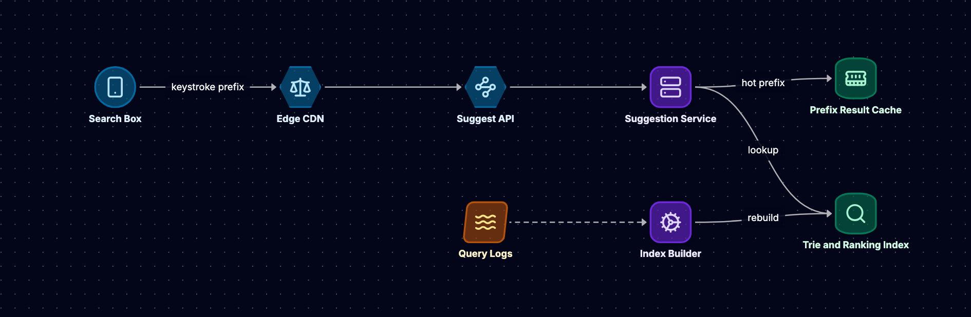
Request Flow: The Critical Path

Before diving into individual components, understanding the request flow illuminates why each architectural decision matters. When a user types "java", their keystroke triggers a cascade through multiple system layers, each with strict latency budgets.

Client to Edge: The browser debounces keystrokes (typically 150-200ms) and sends the partial query to the nearest edge server. Geographic distribution matters here. A user in Singapore hitting a US datacenter adds 180ms+ of network latency before any processing begins.

Edge Cache Layer: The edge server checks its local cache first. This L1 cache holds the most popular prefix queries and can serve responses in 1-5ms. Cache hits at this layer are critical for meeting latency targets. For popular queries like "weather", "amazon", or "youtube", hit rates can exceed 40% of total traffic.

Application Tier: On cache miss, the request reaches the application server, which fans out to multiple backend shards in parallel. This is where query parsing, shard selection, and result aggregation happen. The application tier maintains an L2 cache (typically Redis) that's shared across all application servers, providing another defense against backend load.

Data Tier: Each shard searches its portion of the index using either a trie or inverted index structure. Results stream back as soon as they're found. The application server doesn't wait for all shards to respond; it can return results from the fastest shards and cancel slow requests (hedged requests pattern).

Ranking and Personalization: Retrieved candidates pass through a ranking pipeline that applies scoring functions based on popularity, recency, user history, and contextual signals. This step must complete in single-digit milliseconds to fit within the overall latency budget.

The entire round trip, from keystroke to rendered suggestions, must complete in under 100ms to feel instantaneous. On a hypothetical system, this budget might break down as: 5ms edge routing, 10ms application processing, 30ms data tier search, 10ms ranking, 5ms serialization, and 40ms network overhead. Every component must be optimized.

Data Structures: Trie vs Inverted Index

The choice between a trie and an inverted index fundamentally shapes your system's characteristics. Both can power autocomplete, but they optimize for different access patterns and scale differently.

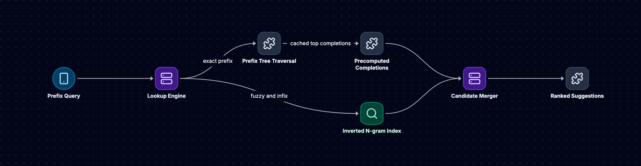
Trie Structure and Performance

A trie (prefix tree) stores strings in a tree where each node represents a character. To find completions for "jav", you traverse j → a → v and enumerate all paths from that node. Tries excel at prefix matching because the traversal naturally finds all strings sharing a prefix.

class TrieNode:
    def __init__(self):
        self.children = {}  # char -> TrieNode
        self.is_end = False
        self.score = 0.0  # popularity/ranking score
        self.top_k = []   # pre-computed top suggestions

class Trie:
    def __init__(self):
        self.root = TrieNode()
    
    def insert(self, word, score):
        node = self.root
        for char in word:
            if char not in node.children:
                node.children[char] = TrieNode()
            node = node.children[char]
        node.is_end = True
        node.score = score

The key optimization is pre-computing top-k suggestions at each node. When inserting "javascript", you update the top-k list at every node along the path (j, ja, jav, etc.) with this term if its score warrants inclusion. At query time, you simply traverse to the prefix node and return its pre-computed top-k list in O(prefix length) time.

Memory consumption is the primary constraint. A trie storing English words might use 50-100 bytes per node (8 bytes for pointers, 8 for score, plus top-k storage). For a corpus of 10 million unique strings with average length 15 characters, you might need 15 billion nodes in the worst case. In practice, prefix sharing reduces this significantly, but a naive trie can still consume 50-100GB for a moderately sized corpus.

Compressed tries (radix trees) merge chains of single-child nodes, reducing memory by 40-60%. Instead of storing "j" → "a" → "v" → "a" as four nodes, you store "java" as one node with a string label. This trades some insertion complexity for substantial memory savings.

Inverted Index Approach

An inverted index maps terms to document IDs (or in this case, suggestion IDs). For autocomplete, you generate all prefixes of each term and index them. The term "javascript" generates prefixes: j, ja, jav, java, javas, etc., each mapping to "javascript".

class InvertedIndex:
    def __init__(self):
        self.index = {}  # prefix -> list[(term, score)]
    
    def add_term(self, term, score):
        for i in range(1, len(term) + 1):
            prefix = term[:i]
            if prefix not in self.index:
                self.index[prefix] = []
            self.index[prefix].append((term, score))

Inverted indexes integrate naturally with existing search infrastructure (Elasticsearch, Solr). You can leverage mature tokenization, scoring, and distributed search capabilities. The data structure is also simpler to update incrementally: adding a new term doesn't require tree rebalancing.

The tradeoff is query-time cost. For a prefix with thousands of matches, you must retrieve, deduplicate, and sort the candidate list on every request. While tries pre-compute top-k at index time, inverted indexes do more work at query time. Mitigations include caching sorted results for popular prefixes and limiting the candidate set size retrieved from the index.

Which to Choose?

Use a trie when: (1) Your corpus is relatively static or updates happen in batch, (2) Memory is available for pre-computation, (3) You need predictable single-digit millisecond latency, (4) Your queries are primarily prefix-based.

Use an inverted index when: (1) You already have search infrastructure like Elasticsearch, (2) Your corpus updates frequently with millions of changes daily, (3) You need fuzzy matching or complex query support, (4) You want to avoid maintaining custom data structures.

Many production systems use both: tries for the hottest prefixes (cached in memory), inverted indexes for the long tail. This hybrid approach balances latency for common queries with flexibility for rare ones.

Sharding and Replication for Low Latency

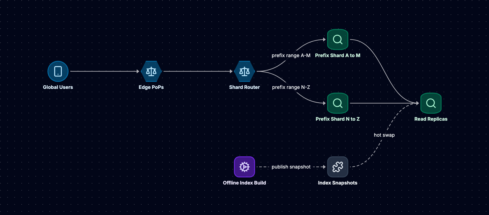
A single server cannot hold a billion-document corpus in memory or serve 100,000 queries per second. Sharding distributes data across machines, while replication provides redundancy and increases read capacity. The sharding strategy directly impacts latency, load distribution, and operational complexity.

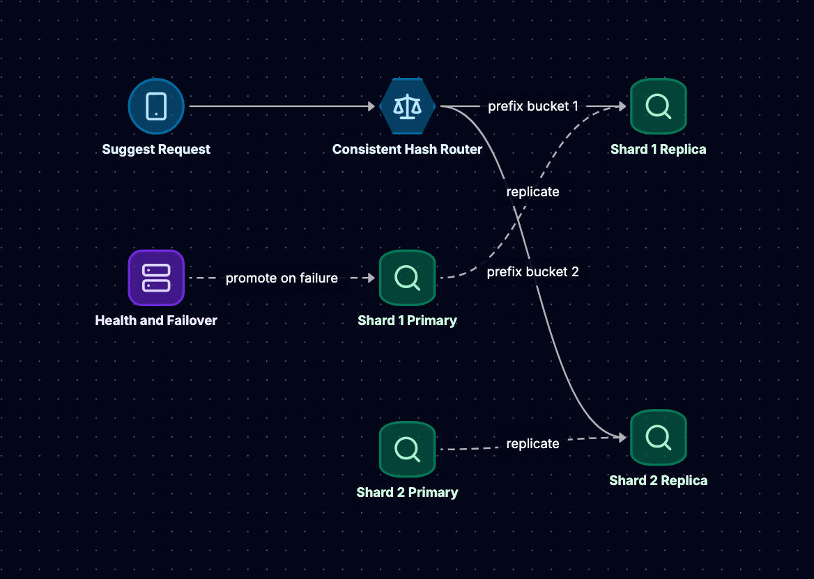
Sharding Strategies

Term-based sharding partitions data by the term itself, typically using consistent hashing. Terms starting with "a-c" go to shard 1, "d-f" to shard 2, etc. This approach has a critical flaw for autocomplete: queries for popular prefixes like "a" or "s" hit only one shard, creating hot spots. Shard 1 handles all queries starting with "a", while other shards sit idle.

Prefix-based sharding assigns different prefixes to different shards based on query volume. High-traffic prefixes like "am" (amazon, american, etc.) get dedicated shards, while low-traffic prefixes share shards. This balances load better but requires monitoring and rebalancing as query patterns shift.

Geographic sharding partitions data by user location or language. US English queries hit US shards, UK English hits UK shards. This reduces latency by keeping data close to users and naturally segments the corpus by regional relevance (users in India care more about "cricket" than "baseball").

class ShardRouter:
    def __init__(self, shard_map):
        self.shard_map = shard_map  # prefix -> shard_ids
    
    def route_query(self, prefix, user_context):
        # Example: route based on prefix and geography
        base_shards = self.shard_map.get(prefix[:2], [0])
        geo_shard = self.get_geo_shard(user_context.country)
        return base_shards + [geo_shard]
    
    def get_geo_shard(self, country):
        # Route to geographically appropriate shard
        geo_map = {'US': 10, 'UK': 11, 'IN': 12}
        return geo_map.get(country, 10)

The router fans out queries to multiple shards in parallel. For a query "java", it might query 3-5 shards simultaneously, collect results, merge and rank them, and return the top-k. Parallel fan-out means latency equals the slowest shard response, not the sum of all shards.

Replication for Availability and Throughput

Each shard typically has 3-5 replicas distributed across availability zones. Replication serves two purposes: fault tolerance (if one replica fails, others serve traffic) and load distribution (read queries spread across replicas).

The application tier maintains a replica health map. When a replica becomes slow or unhealthy, the router stops sending it traffic. Health checks run continuously, measuring response times and error rates. A replica consistently responding slower than peers gets marked degraded and receives reduced traffic.

Hedged requests further reduce tail latency. After sending a request to one replica, if no response arrives within a threshold (perhaps 50ms for illustration), send the same request to a second replica. Return whichever responds first and cancel the other. This technique can cut p99 latency in half by avoiding stragglers, at the cost of increased backend load.

Handling Shard Failures

When a shard goes down, its replicas handle the load. But what if all replicas of a shard fail? You have two options:

1. Degrade gracefully: Return partial results from available shards. For autocomplete, showing 7 suggestions instead of 10 is acceptable. The system remains available even if 20% of shards are down.

2. Failover to backup: Maintain cold standbys that can be promoted. This increases infrastructure cost but provides full coverage.

Most systems choose graceful degradation for autocomplete. Unlike search results, where missing critical documents is unacceptable, autocomplete can function with reduced suggestion quality during incidents.

Ranking and Personalization

Retrieving candidate suggestions is only half the problem. Ranking them relevantly is what makes autocomplete useful. A naive alphabetical sort is useless; users expect popular, relevant suggestions first. Ranking combines global popularity signals with personalized relevance.

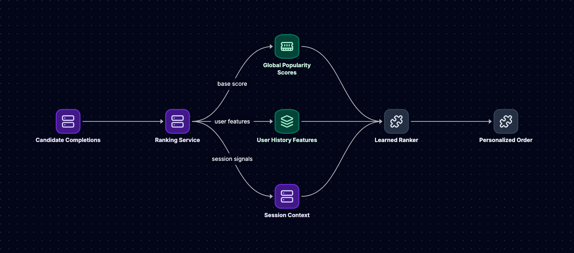
Global Popularity Signals

Query frequency is the foundational signal. Terms users search for often should rank higher. Track query counts in a time-decayed manner so recent popularity matters more than historical. A simple exponential decay model:

import math
from datetime import datetime, timedelta

class PopularityScorer:
    def __init__(self, half_life_days=7):  # Example parameter
        self.half_life = half_life_days * 86400
        self.counts = {}  # term -> (count, last_update)
    
    def record_query(self, term, timestamp):
        if term in self.counts:
            old_count, old_time = self.counts[term]
            decay = math.exp(-0.693 * (timestamp - old_time) / self.half_life)
            new_count = old_count * decay + 1.0
        else:
            new_count = 1.0
        self.counts[term] = (new_count, timestamp)
    
    def get_score(self, term, current_time):
        if term not in self.counts:
            return 0.0
        count, last_update = self.counts[term]
        decay = math.exp(-0.693 * (current_time - last_update) / self.half_life)
        return count * decay

This model gives recent queries more weight. A query searched 1000 times last week scores higher than one searched 1000 times six months ago. The half-life parameter controls how quickly popularity decays (requires tuning for specific use case).

Click-through rate refines popularity. If users select "java tutorial" 80% of the time it's shown but "java coffee" only 10%, "java tutorial" should rank higher even if both appear in query logs equally. Track impressions and clicks separately, then compute CTR.

Conversion rate goes further: did the user find what they wanted? If 50% of users who select "java tutorial" immediately bounce back, that suggestion isn't truly helpful. Tracking downstream engagement (clicks on results, time on site, purchases) provides a quality signal beyond raw popularity.

Personalization Signals

Generic rankings work for most users, but personalization can significantly improve relevance. A developer typing "python" wants programming content; a pet owner wants snake care information.

User history is the most direct signal. If a user previously searched for "python tutorial", "django", and "flask", they're clearly interested in programming. Weight suggestions matching their historical interests higher. Store recent queries (last 30 days) and extract topics or categories.

class PersonalizedRanker:
    def __init__(self):
        self.user_profiles = {}  # user_id -> interest_vector
    
    def build_profile(self, user_id, query_history):
        # Extract topics from historical queries
        topics = self.extract_topics(query_history)
        self.user_profiles[user_id] = topics
    
    def score(self, user_id, suggestion, base_score):
        if user_id not in self.user_profiles:
            return base_score
        
        profile = self.user_profiles[user_id]
        suggestion_topics = self.extract_topics([suggestion])
        
        # Compute overlap between user interests and suggestion
        overlap = self.compute_overlap(profile, suggestion_topics)
        personalization_boost = 1.0 + (0.3 * overlap)  # Example boost
        return base_score * personalization_boost

Contextual signals include time of day, location, device type, and session behavior. A user searching at 8am on mobile might want different results than at 8pm on desktop. Location enables local suggestions: "pizza" should surface nearby restaurants, not the Wikipedia article.

Collaborative filtering leverages patterns across users. If users similar to you (based on search history) frequently select "java spring boot" after typing "java", that suggestion ranks higher for you too. This cold-starts personalization for new users by borrowing signals from similar users.

Combining Signals: The Scoring Function

A production ranking function combines dozens of signals. A simplified example:

def rank_suggestions(candidates, user_context, global_stats):
    scored = []
    for suggestion in candidates:
        # Combine multiple signals with learned or tuned weights
        score = (
            0.4 * global_stats.popularity(suggestion) +  # Example weights
            0.2 * global_stats.ctr(suggestion) +
            0.2 * personalization_score(user_context, suggestion) +
            0.1 * recency_score(suggestion) +
            0.1 * contextual_score(user_context, suggestion)
        )
        scored.append((suggestion, score))
    
    scored.sort(key=lambda x: x[1], reverse=True)
    return [s[0] for s in scored[:10]]

The weights (0.4, 0.2, etc.) require tuning through A/B testing. Start with intuition, then iterate based on metrics like CTR, user engagement, and conversion. Machine learning models (gradient boosted trees, neural networks) can learn these weights automatically from labeled data, but even simple weighted combinations work well with proper tuning.

Ranking must execute in milliseconds. Pre-compute expensive features (popularity, CTR) offline and store them with the index. At query time, only compute cheap features (personalization, contextual) that depend on the specific request.

Index Build and Refresh Pipeline

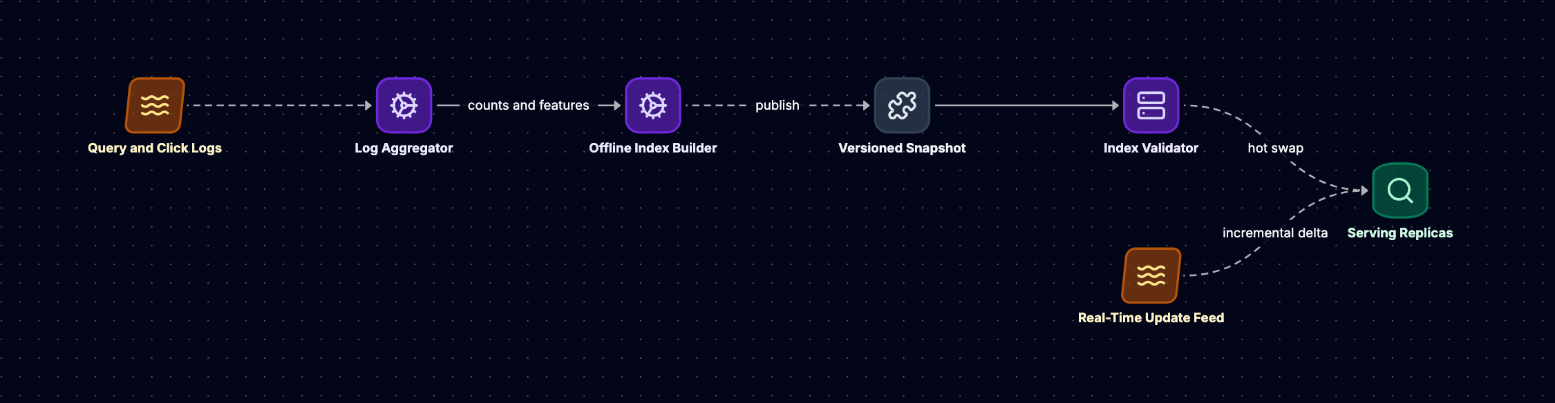
Autocomplete indexes must stay current as new content appears and popularity shifts. A news site needs breaking stories in autocomplete within minutes. An e-commerce site needs new products searchable immediately. The index pipeline ingests updates, rebuilds indexes, and deploys them without downtime.

Batch vs Streaming Updates

Batch rebuilds regenerate the entire index periodically (hourly, daily). This approach is simple: dump the latest corpus, build a new trie or inverted index, and swap it in atomically. Batch rebuilds work well for relatively static corpora or when freshness requirements are relaxed (daily updates acceptable).

The downside is latency: updates don't appear until the next rebuild completes. For a large corpus, building a new index might take 30-60 minutes. During that window, new content isn't searchable.

Streaming updates apply incremental changes continuously. As new documents arrive, insert them into the live index. As documents are deleted or updated, remove or modify their entries. Streaming provides near-real-time freshness (seconds to minutes) but adds complexity.

class StreamingIndexUpdater:
    def __init__(self, index):
        self.index = index
        self.update_queue = []
    
    def enqueue_update(self, operation, term, score):
        self.update_queue.append((operation, term, score))
    
    def apply_updates(self):
        # Process updates in batches for efficiency
        for op, term, score in self.update_queue:
            if op == 'INSERT':
                self.index.add_term(term, score)
            elif op == 'DELETE':
                self.index.remove_term(term)
            elif op == 'UPDATE':
                self.index.update_score(term, score)
        self.update_queue.clear()

Tries are harder to update incrementally than inverted indexes. Inserting a new term into a trie requires traversing and potentially updating top-k lists at every node along the path. For high-frequency updates, this becomes expensive. Inverted indexes simply append to posting lists, making incremental updates cheaper.

Popularity Decay and Recomputation

Popularity scores decay over time. Yesterday's trending topic shouldn't dominate autocomplete forever. Recompute scores periodically (hourly or daily) based on recent query logs.

A typical pipeline:

1. Log aggregation: Collect query logs from all application servers into a central store (S3, HDFS).

2. Score computation: Run a batch job (Spark, MapReduce) to count queries, compute CTR, apply time decay, and generate updated scores for all terms.

3. Index update: Feed updated scores back into the index. For batch rebuilds, this happens during the full rebuild. For streaming, push score updates through the update queue.

4. Deployment: Atomically switch traffic to the new index once updates are applied.

This pipeline runs continuously. Fresh query logs arrive every few minutes, score computation runs hourly, and index updates deploy as soon as they're ready.

Blue-Green Deployment for Zero Downtime

You cannot take down autocomplete to deploy a new index. Use blue-green deployment: maintain two complete index clusters (blue and green). Build the new index on the inactive cluster, validate it, then switch traffic.

1. Blue cluster serves production traffic.
2. Build new index on green cluster.
3. Run validation queries to ensure green cluster returns expected results.
4. Flip load balancer to route traffic to green.
5. Blue becomes the inactive cluster, ready for the next update.

If the new index has issues, roll back by flipping traffic back to blue. This pattern provides instant rollback capability and zero downtime during deployments.

Handling Schema Changes

Occasionally, you need to change the index schema: add new fields, change tokenization, or modify scoring logic. Schema changes require full rebuilds. Plan these carefully:

1. Build new indexes with the new schema in parallel with old indexes.
2. Run both old and new indexes simultaneously, comparing results.
3. Gradually shift traffic to new indexes (10%, 50%, 100%) while monitoring metrics.
4. Once confident, decommission old indexes.

This gradual migration reduces risk. If the new schema degrades quality, you catch it at 10% traffic, not 100%.

Caching Tiers and Cache Invalidation

Caching is critical for meeting latency targets and reducing backend load. A well-designed cache hierarchy can serve 80-90% of requests without touching the data tier. But caching introduces complexity: stale data, cache invalidation, and memory management.

L1: Edge Cache

The first cache tier sits at the edge, closest to users. Edge servers (CDN nodes, regional POPs) cache popular queries locally. This cache has the lowest latency (1-5ms) but limited capacity (1-10GB per node).

What to cache: Only the most popular prefixes. Queries like "weather", "youtube", "facebook" account for a disproportionate share of traffic. A small cache holding the top 10,000 prefixes can serve 30-50% of requests.

TTL strategy: Short TTLs (1-5 minutes) keep data fresh. Autocomplete suggestions change frequently as popularity shifts. A 5-minute TTL means suggestions are at most 5 minutes stale, acceptable for most use cases.

Cache warming: Pre-populate edge caches with popular queries during deployment. Don't wait for cache misses to populate the cache. This avoids a thundering herd when a new edge node comes online.

L2: Application Cache

The second tier sits at the application layer, typically using Redis or Memcached. This cache is shared across all application servers, providing a larger capacity (100GB - 1TB) and lower latency than the data tier (5-20ms).

class CacheLayer:
    def __init__(self, l1_cache, l2_cache, data_tier):
        self.l1 = l1_cache  # Local in-memory cache
        self.l2 = l2_cache  # Shared Redis cache
        self.data_tier = data_tier
    
    def get_suggestions(self, prefix, user_context):
        # Try L1 first
        key = self.build_cache_key(prefix, user_context)
        result = self.l1.get(key)
        if result:
            return result
        
        # Try L2
        result = self.l2.get(key)
        if result:
            self.l1.set(key, result, ttl=60)  # Example TTL
            return result
        
        # Query data tier
        result = self.data_tier.query(prefix, user_context)
        self.l2.set(key, result, ttl=300)  # Example TTL
        self.l1.set(key, result, ttl=60)
        return result

Personalization and caching: Personalized results are harder to cache because each user gets different suggestions. Strategies include: (1) Cache only the non-personalized base results, then apply personalization at query time, (2) Cache personalized results with user ID in the cache key, accepting lower hit rates, (3) Segment users into cohorts and cache per-cohort results.

L3: Data Tier Cache

The data tier itself often has caching (OS page cache, database buffer pool). This cache is transparent to the application but significantly impacts performance. Ensure hot data (popular prefixes, recent updates) stays in memory.

For a trie-based system, frequently accessed nodes should remain in memory. Use memory-mapped files or an in-memory database to keep the working set resident. For inverted indexes, database query caches and posting list caches serve a similar role.

Cache Invalidation: The Hard Problem

Phil Karlton famously said, "There are only two hard things in Computer Science: cache invalidation and naming things." Cache invalidation for autocomplete is particularly tricky because data changes frequently.

Time-based invalidation (TTL): The simplest approach. Set a TTL (1-5 minutes for edge, 5-30 minutes for L2) and let caches expire naturally. This works well when freshness requirements are relaxed and you can tolerate stale data for the TTL duration.

Event-based invalidation: When the index updates, explicitly invalidate affected cache entries. If "java spring boot" gets a popularity boost, invalidate all caches containing "j", "