Choosing the Right Database: A Deep Dive into Six Database Paradigms
Introduction
In a system design interview, the question "Which database would you use?" separates candidates who memorize buzzwords from those who understand trade-offs. The right answer isn't PostgreSQL or MongoDB or Cassandra: it's "It depends on the access patterns, consistency requirements, and scale."
This post gives senior backend engineers the depth needed to choose and defend a database architecture. We'll examine six paradigms (relational, document, key-value, wide-column, graph, and time-series) through a consistent lens: how they store data internally, how they scale, where they excel, and where they fail. We'll model the same domain (users, orders, products, social connections, and metrics) in each system, then provide a decision framework for three concrete scenarios.
By the end, you'll be able to explain why a checkout service and a sensor pipeline deserve different databases, and defend either choice in an interview without falling into the "NoSQL scales, SQL doesn't" trap.
Relational Databases: PostgreSQL and Aurora
When to Reach for SQL
Relational databases dominate when you need strong consistency guarantees and complex queries across normalized data. They remain the default choice for most new systems, and for good reason: when your business logic requires multi-row transactions (think e-commerce checkout: decrement inventory, create order, charge payment), ACID semantics prevent your system from losing money.
PostgreSQL represents the open-source gold standard. Aurora is AWS's cloud-native fork that separates compute from storage, claiming higher availability and read scaling through replicas that share the same storage layer.
Trade-offs: You get correctness and query flexibility at the cost of vertical scaling limits and operational complexity when you need horizontal writes. A well-tuned single primary on modern hardware serves a very large share of real-world workloads, and read replicas stretch reads further. Writes are the ceiling: every write goes through one primary, and once that saturates you shard, which breaks cross-shard transactions and joins.
How Relational Storage Works
PostgreSQL stores data in 8KB pages organized into heap files. Each table is a collection of pages; each row is a tuple within a page. Indexes (B-tree by default) map search keys to page locations. When you query SELECT * FROM orders WHERE user_id = 123, PostgreSQL:
- Consults the B-tree index on
user_id - Retrieves matching tuple IDs (TIDs)
- Fetches pages from disk (or buffer cache)
- Applies MVCC (Multi-Version Concurrency Control) to return only rows visible to your transaction
MVCC is why PostgreSQL handles concurrent reads and writes without locking: each transaction sees a snapshot. Dead tuples accumulate until VACUUM reclaims space.
Transactions guarantee ACID through a write-ahead log (WAL). Before committing, PostgreSQL writes all changes to WAL on disk. If the server crashes, it replays the log on restart. Serializable isolation (the strictest level) uses predicate locks to prevent anomalies, but at a latency cost.
Modeling Our Domain
CREATE TABLE users (
  user_id SERIAL PRIMARY KEY,
  username VARCHAR(50) UNIQUE NOT NULL,
  email VARCHAR(255) UNIQUE NOT NULL,
  created_at TIMESTAMP DEFAULT NOW()
);

CREATE TABLE products (
  product_id SERIAL PRIMARY KEY,
  name VARCHAR(255) NOT NULL,
  price NUMERIC(10,2) NOT NULL,
  stock INT NOT NULL
);

CREATE TABLE orders (
  order_id SERIAL PRIMARY KEY,
  user_id INT REFERENCES users(user_id),
  total NUMERIC(10,2) NOT NULL,
  status VARCHAR(20) NOT NULL,
  created_at TIMESTAMP DEFAULT NOW()
);

CREATE TABLE order_items (
  order_id INT REFERENCES orders(order_id),
  product_id INT REFERENCES products(product_id),
  quantity INT NOT NULL,
  price NUMERIC(10,2) NOT NULL,
  PRIMARY KEY (order_id, product_id)
);

CREATE INDEX idx_orders_user ON orders(user_id);
CREATE INDEX idx_orders_created ON orders(created_at);
A checkout transaction:
BEGIN;
  -- Check stock
  SELECT stock FROM products WHERE product_id = 456 FOR UPDATE;
  -- Decrement
  UPDATE products SET stock = stock - 1 WHERE product_id = 456;
  -- Create order
  INSERT INTO orders (user_id, total, status) VALUES (123, 29.99, 'pending');
  -- Insert line item
  INSERT INTO order_items (order_id, product_id, quantity, price)
    VALUES (currval('orders_order_id_seq'), 456, 1, 29.99);
COMMIT;
The FOR UPDATE row lock prevents double-selling. If the transaction aborts, all changes roll back atomically.
Scaling Relational Databases
Vertical scaling (bigger machines) is the primary path, and it goes further than most people assume: a single large instance with enough RAM to hold the working set covers most applications. When you exhaust vertical headroom:
- Read replicas handle read traffic. Aurora's architecture allows up to 15 replicas sharing the same storage, reducing replication lag. Standard PostgreSQL replication is asynchronous (lag of milliseconds to seconds) or synchronous (higher latency, guaranteed durability).
- Connection pooling (PgBouncer) multiplexes thousands of client connections onto a smaller pool of database connections, reducing overhead.
- Sharding splits data across independent databases. You pick a shard key (e.g.,
user_id % 16) and route queries. Cross-shard joins and transactions break; you handle them in application code or accept eventual consistency.
Joins are cheap when they hit indexes and expensive when they don't; a many-table join over large, poorly indexed tables is where query plans fall apart. Denormalization (duplicating data to avoid joins) trades storage and update complexity for read speed.
Failure Modes and Anti-Patterns
- N+1 queries: Fetching a list of orders, then looping to fetch each user separately. Use
JOINor batch the second query. - Missing indexes: Full table scans on large tables.
EXPLAIN ANALYZEshows sequential scans; add indexes on filter and join columns. - Lock contention: High-concurrency updates to the same rows (e.g., incrementing a global counter). Use optimistic locking or move counters to Redis.
- Vacuum bloat: Infrequent vacuuming causes table bloat and index bloat, degrading performance. Tune autovacuum or run manual
VACUUM. - Connection exhaustion: Each PostgreSQL backend is a process. Default max_connections is 100. Going higher increases memory overhead. Use pooling.
Document Databases: MongoDB
When JSON Fits Your Domain
Document databases shine when your entities are hierarchical and semi-structured, and you rarely need to query across entity boundaries. The appeal is development speed: the stored shape matches the object in your code, and adding a field needs no migration.
MongoDB stores BSON (binary JSON) documents in collections. Each document is self-contained, so fetching a user profile with nested addresses and preferences is a single read, not a join across three tables. Data that is read together is stored together.
Trade-offs: You denormalize aggressively, duplicating data. Updates to shared data (e.g., a product name appearing in thousands of order documents) require bulk updates. Multi-document transactions arrived in MongoDB 4.0 (replica sets) and 4.2 (sharded clusters), but they carry a performance cost and are not the model the database is optimized for.
How Document Storage Works
MongoDB organizes data into collections (analogous to tables) of documents (analogous to rows, but schema-free). Internally, documents are stored in a B-tree-based storage engine (WiredTiger by default). Each document has a unique _id (auto-generated ObjectId or custom).
Indexes accelerate queries. MongoDB supports single-field, compound, multikey (for arrays), geospatial, and text indexes. An index on { user_id: 1, created_at: -1 } speeds up queries filtering by user and sorting by date.
Replication uses a primary-secondary model. Writes go to the primary; secondaries replicate asynchronously. If the primary fails, an election promotes a secondary. Since MongoDB 5.0 the default write concern is w: majority, which waits for a majority of nodes before acknowledging; dropping to w: 1 acknowledges after the primary alone, trading durability on failover for lower latency.
Sharding distributes collections across shards (replica sets). You pick a shard key (e.g., user_id). MongoDB routes queries based on the key. Choosing a poor shard key (e.g., monotonically increasing _id) creates hotspots: all writes hit one shard.
Modeling Our Domain
// users collection
{
  _id: ObjectId("507f1f77bcf86cd799439011"),
  username: "alice",
  email: "alice@example.com",
  created_at: ISODate("2023-01-15T10:30:00Z")
}

// products collection
{
  _id: ObjectId("507f1f77bcf86cd799439012"),
  name: "Laptop",
  price: 999.99,
  stock: 50
}

// orders collection (denormalized)
{
  _id: ObjectId("507f1f77bcf86cd799439013"),
  user_id: ObjectId("507f1f77bcf86cd799439011"),
  user_name: "alice",  // denormalized for display
  total: 999.99,
  status: "shipped",
  created_at: ISODate("2023-02-20T14:22:00Z"),
  items: [
    {
      product_id: ObjectId("507f1f77bcf86cd799439012"),
      product_name: "Laptop",  // denormalized
      quantity: 1,
      price: 999.99
    }
  ]
}
Fetching an order with all details:
db.orders.findOne({ _id: ObjectId("507f1f77bcf86cd799439013") })
One query returns everything. In PostgreSQL, you'd join orders, order_items, products, and users.
Creating an order (without multi-document transactions):
// 1. Check stock (race condition possible)
const product = db.products.findOne({ _id: productId });
if (product.stock < 1) throw new Error("Out of stock");

// 2. Decrement stock
db.products.updateOne(
  { _id: productId, stock: { $gte: 1 } },
  { $inc: { stock: -1 } }
);

// 3. Insert order
db.orders.insertOne({
  user_id: userId,
  user_name: "alice",
  total: 999.99,
  status: "pending",
  items: [{ product_id: productId, product_name: "Laptop", quantity: 1, price: 999.99 }],
  created_at: new Date()
});
The stock: { $gte: 1 } condition prevents overselling if concurrent requests race, but this isn't a true transaction. If the insert fails, stock is decremented anyway. For strong consistency, wrap in a multi-document transaction (available in MongoDB 4.0+), accepting higher latency.
Scaling MongoDB
Read scaling: Add secondaries to the replica set. Configure read preference to secondary or nearest for eventually consistent reads. Primary handles all writes.
Write scaling: Shard the collection. Choose a shard key with high cardinality and even distribution. For orders, user_id works if users are evenly distributed. Avoid created_at alone (all writes hit the newest chunk). A compound key like { user_id: 1, created_at: 1 } balances distribution and query efficiency.
Indexing strategy: MongoDB loads indexes into RAM. If indexes exceed RAM, performance degrades. Monitor working set size and scale RAM accordingly.
Failure Modes and Anti-Patterns
- Unbounded arrays: Embedding all orders in a user document grows the document indefinitely. MongoDB's 16MB document limit will be hit. Use references or a separate collection.
- Poor shard key: Monotonic keys (e.g.,
_id,created_at) create hotspots. All writes target one shard until it splits. Choose a key that distributes writes evenly. - Scatter-gather queries: Queries without the shard key hit all shards, then merge results. Latency multiplies. Design queries to include the shard key.
- Missing indexes on large collections: Without an index, MongoDB scans all documents. Add indexes on frequently queried fields.
- Overusing transactions: Multi-document transactions lock documents and increase latency. Use them sparingly; design for single-document atomicity where possible.
Key-Value Stores: DynamoDB and Redis
When Simple and Fast Wins
Key-value stores are the simplest paradigm: a distributed hash map. You put a value at a key, you get it back. Because every operation is addressed by key, the database never plans a query: it hashes the key, finds the owner, and reads. That is why in-memory stores like Redis answer in well under a millisecond and why DynamoDB keeps single-digit millisecond latency regardless of table size.
Redis is an in-memory data structure server. Beyond strings, it supports lists, sets, sorted sets, hashes, bitmaps, and more. Persistence is optional (RDB snapshots or AOF logs). Use it for caching, session storage, leaderboards, rate limiting, and pub/sub.
DynamoDB is AWS's managed key-value and document store (it supports nested JSON). It auto-scales to millions of requests per second and stores petabytes. You pay per request and storage, avoiding operational overhead.
Trade-offs: You lose query flexibility. No joins, no secondary indexes without cost (DynamoDB global secondary indexes consume additional throughput), no complex filtering. Data modeling is denormalization on steroids: you precompute access patterns and store results.
How Key-Value Storage Works
Redis stores data in RAM in a hash table. Each key maps to a value (string, list, set, etc.). Eviction policies (LRU, LFU) remove keys when memory fills. Persistence options:
- RDB: Periodic snapshots. Fast, compact, but loses data between snapshots.
- AOF: Append-only log of every write. Durable, but larger and slower to load.
Redis is single-threaded for command execution (I/O is multiplexed via epoll/kqueue), so operations are atomic. Complex operations (e.g., incrementing a counter) don't require transactions.
DynamoDB stores data in partitions (10GB each). Partition key hashes determine placement. Within a partition, items are sorted by sort key (optional). DynamoDB replicates across three availability zones synchronously.
Reads are eventually consistent by default (lower latency) or strongly consistent (higher latency, reads from the leader). Writes go to the partition's leader and acknowledge once two of the three replicas have durably logged them.
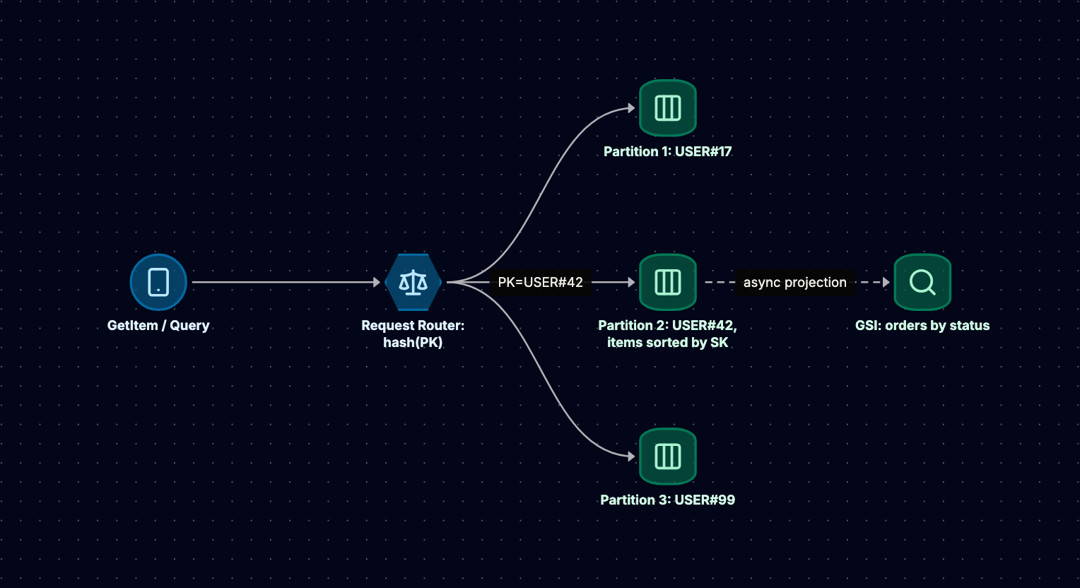
Global secondary indexes (GSI) let you query by non-key attributes. Each GSI is a separate table with its own partition key, consuming additional read/write capacity.
Modeling Our Domain
Redis (session cache):
# Store session
SET session:a1b2c3d4 '{"user_id":123,"username":"alice","expires":1672531200}' EX 3600

# Retrieve session
GET session:a1b2c3d4

# Leaderboard (sorted set)
ZADD leaderboard:2023-02 1500 "alice"
ZADD leaderboard:2023-02 1450 "bob"
ZREVRANGE leaderboard:2023-02 0 9 WITHSCORES  # Top 10

# Rate limiting (counter with expiry)
INCR rate_limit:user:123:2023-02-20:14
EXPIRE rate_limit:user:123:2023-02-20:14 3600
DynamoDB (orders table):
// Table: Orders
// Partition key: user_id
// Sort key: order_id

PutItem({
  TableName: "Orders",
  Item: {
    user_id: "123",
    order_id: "20230220-a1b2c3",
    total: 999.99,
    status: "shipped",
    created_at: "2023-02-20T14:22:00Z",
    items: [
      { product_id: "456", product_name: "Laptop", quantity: 1, price: 999.99 }
    ]
  }
});

// Query all orders for a user
Query({
  TableName: "Orders",
  KeyConditionExpression: "user_id = :uid",
  ExpressionAttributeValues: { ":uid": "123" }
});

// Get a specific order
GetItem({
  TableName: "Orders",
  Key: { user_id: "123", order_id: "20230220-a1b2c3" }
});
To query orders by status, you'd create a GSI with status as the partition key and created_at as the sort key. This duplicates data and consumes extra capacity, but enables the query.
Scaling Key-Value Stores
Redis scaling:
- Vertical: Increase memory. Redis Enterprise and cloud providers offer instances with hundreds of GB.
- Horizontal: Redis Cluster shards data across nodes. The cluster specification targets up to about 1,000 nodes. Each key hashes to one of 16,384 slots, distributed across nodes. Clients route requests directly to the correct node.
- Read replicas: Each primary can have replicas. Replicas serve reads, reducing primary load.
DynamoDB scaling: DynamoDB has no practical table-level throughput ceiling, but each partition does (roughly 3,000 read units and 1,000 write units per second). You provision read/write capacity units (RCU/WCU) or use on-demand mode (pay per request). DynamoDB splits partitions automatically when they exceed throughput or storage limits. Avoid hot keys: if one partition key receives disproportionate traffic, it throttles.
Failure Modes and Anti-Patterns
- Hot keys in Redis: One key receiving millions of requests per second. Redis is single-threaded; one slow operation blocks others. Solution: shard the key (e.g.,
counter:0,counter:1, ...,counter:9) and aggregate. - Cache stampede: Cache expires, many requests hit the database simultaneously. Use locking or probabilistic early expiration.
- DynamoDB hot partition: Uneven access patterns throttle one partition. Use a composite partition key or add randomness (write sharding).
- Unbounded item size: DynamoDB's item size limit is 400KB. Storing large blobs (e.g., images) directly fails. Store in S3 and reference the URL.
- GSI propagation lag: GSIs update asynchronously. After writing, a query on a GSI may not reflect the write immediately. Design for eventual consistency or use the base table.
Wide-Column Stores: Cassandra
When Writes Dominate and Scale is Massive
Wide-column databases optimize for high write throughput and horizontal scalability. Throughput grows close to linearly as you add nodes, which is why companies such as Netflix and Apple have run Cassandra fleets in the thousands of nodes.
Cassandra's architecture is leaderless: every node is equal, eliminating single points of failure. Use it for append-heavy event data, IoT sensor streams, message history (Instagram and Discord both built on it; Discord later moved to the Cassandra-compatible ScyllaDB), and any workload where writes vastly outnumber reads and the queries are known in advance.
Trade-offs: Query flexibility is limited. You design tables for specific queries (query-first modeling). Joins don't exist; you denormalize. Consistency is tunable, not guaranteed: you choose between low latency and strong consistency per query.
How Wide-Column Storage Works
Cassandra's data model has keyspaces (databases), tables, rows, and columns. Each row is identified by a partition key. Rows with the same partition key are stored together on disk, sorted by clustering columns.
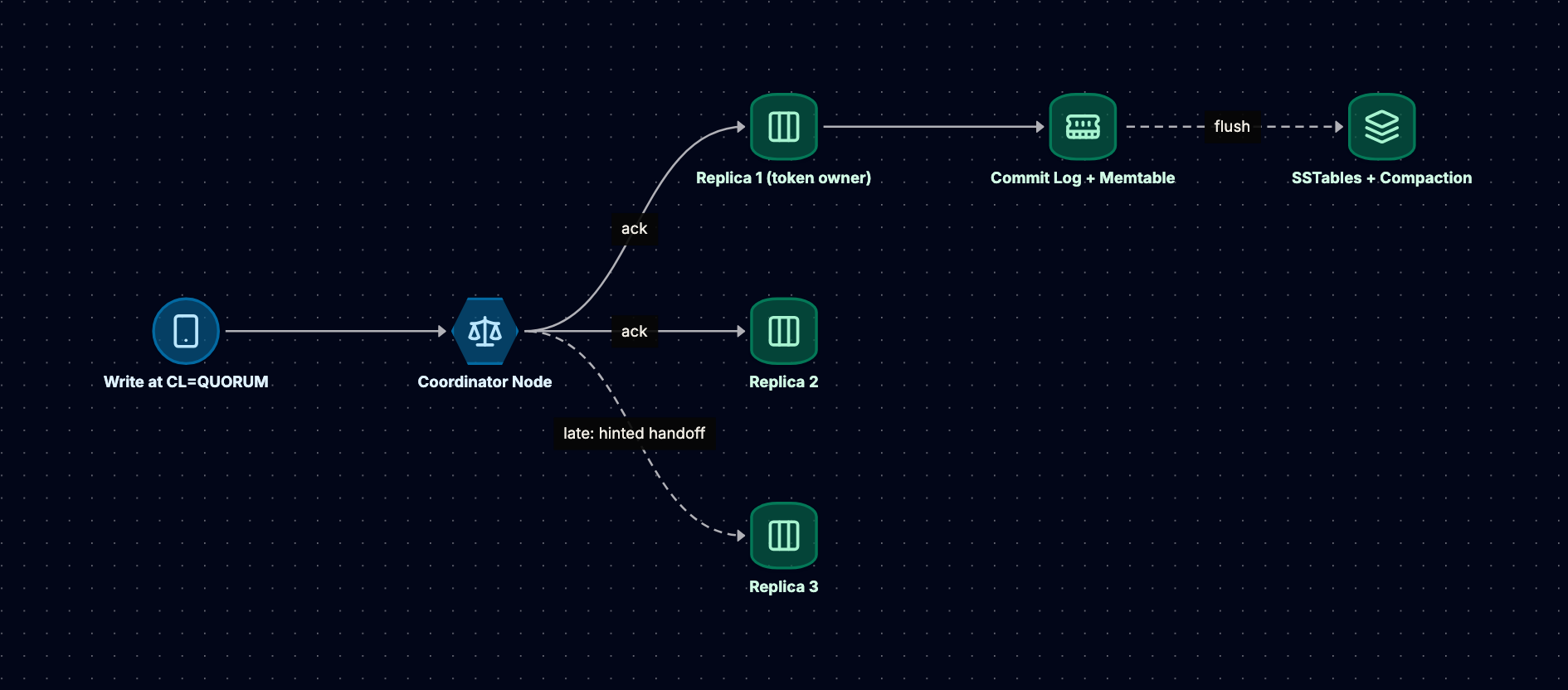
Write path:
- Write to commit log (append-only, on disk) for durability.
- Write to memtable (in-memory sorted structure).
- When memtable fills, flush to SSTable (immutable sorted file on disk).
Writes are fast because they're sequential (commit log) and in-memory (memtable). No read-before-write, no locking.
Read path:
- Check memtable.
- Check row cache (if enabled).
- Consult bloom filters (probabilistic data structure) to skip SSTables that don't contain the key.
- Read from SSTables, merge results.
Compaction merges SSTables periodically, removing deleted data (tombstones) and consolidating updates.
Replication: Data replicates to N nodes (replication factor, typically 3). Partition key hashes to a token; the ring assigns tokens to nodes. Writes go to all replicas. Consistency level determines how many replicas must acknowledge:
ONE: Fastest, least durable.QUORUM: Majority (N/2 + 1), balances latency and consistency.ALL: Slowest, most durable.
Tunable consistency: For strong consistency, use QUORUM for both reads and writes (or LOCAL_QUORUM within a datacenter). This satisfies the quorum intersection property: read and write quorums overlap, guaranteeing you read the latest write.
Modeling Our Domain
Query-first design: decide what queries you need, then design tables to serve them.
Query 1: Get all orders for a user, sorted by date.
CREATE TABLE orders_by_user (
  user_id UUID,
  order_id TIMEUUID,
  total DECIMAL,
  status TEXT,
  created_at TIMESTAMP,
  PRIMARY KEY (user_id, order_id)
) WITH CLUSTERING ORDER BY (order_id DESC);

-- Insert
INSERT INTO orders_by_user (user_id, order_id, total, status, created_at)
VALUES (123e4567-e89b-12d3-a456-426614174000, now(), 999.99, 'shipped', toTimestamp(now()));

-- Query
SELECT * FROM orders_by_user WHERE user_id = 123e4567-e89b-12d3-a456-426614174000;
Partition key user_id groups all orders for a user. Clustering column order_id (TIMEUUID) sorts them by time. This query is efficient: one partition read.
Query 2: Get all orders with status "pending".
You can't query by status in the table above (it's not part of the key). Create a second table:
CREATE TABLE orders_by_status (
  status TEXT,
  order_id TIMEUUID,
  user_id UUID,
  total DECIMAL,
  created_at TIMESTAMP,
  PRIMARY KEY (status, order_id)
) WITH CLUSTERING ORDER BY (order_id DESC);
Now you duplicate data: each order is written to both tables. Cassandra has no foreign keys or triggers; your application writes to both.
Query 3: Time-series metrics (IoT sensor data).
CREATE TABLE sensor_metrics (
  sensor_id UUID,
  date DATE,
  timestamp TIMESTAMP,
  temperature DOUBLE,
  humidity DOUBLE,
  PRIMARY KEY ((sensor_id, date), timestamp)
) WITH CLUSTERING ORDER BY (timestamp ASC);
Composite partition key (sensor_id, date) distributes data evenly (each sensor-day is a partition). Clustering by timestamp allows efficient range queries within a day.
Scaling Cassandra
Because there is no leader, adding capacity is mostly an operational exercise rather than a redesign:
- Add nodes: a new node takes ownership of token ranges (with virtual nodes, many small ranges) and streams the matching data from existing replicas. Throughput grows roughly in proportion to node count, as long as partitions are evenly sized.
- Add datacenters: replication is configured per datacenter (
NetworkTopologyStrategy), so you can run active-active across regions and useLOCAL_QUORUMto keep latency local. - Tune consistency per query:
ONEfor a dashboard read that can be slightly stale,LOCAL_QUORUMfor a balance read that cannot.
What does not scale is a bad partition. A single partition lives on its replicas and nowhere else, so one huge or one hot partition caps the whole design no matter how many nodes you add. A common guideline is to keep partitions under roughly 100 MB and well under a few hundred thousand rows.
Failure Modes and Anti-Patterns
- Unbounded partitions: partitioning
messagesbychannel_idalone means a busy channel grows forever. Add a time bucket to the partition key:PRIMARY KEY ((channel_id, bucket), message_id). - Tombstone build-up: deletes and TTL expiries write tombstones, and reads must scan past them until compaction removes them. Queue-like usage (insert, read, delete) is the classic way to make reads slow and eventually fail with tombstone warnings.
- Using
ALLOW FILTERINGor secondary indexes as a crutch: they turn a single-partition lookup into a cluster-wide scan. If you need a new query, build a new table. - Read-before-write logic: Cassandra's speed comes from blind writes. Lightweight transactions (
IF NOT EXISTS) run Paxos and cost several round trips; using them on the hot path removes the reason you chose Cassandra. - Expecting relational semantics: there are no joins, no foreign keys, and batches are not transactions across partitions. Keeping
orders_by_userandorders_by_statusin sync is your application's job.
Graph Databases: Neo4j
When Relationships Are the Data
Some questions are about the connections, not the entities: "which products did people I follow buy last week?", "is this new account two hops from a known fraud ring?", "what is the shortest path between these two services in our dependency graph?". In a relational database each hop is another self-join, and the cost grows with the size of the tables. A graph database stores relationships as first-class records, so each hop costs roughly the same no matter how big the graph is.
Neo4j is the best-known native graph database. It is a good fit for recommendations, fraud and identity resolution, network and dependency analysis, access-control graphs, and knowledge graphs.
Trade-offs: excellent at traversals from a known starting point, mediocre at everything else. Large aggregations ("total revenue by month") and bulk scans are better served elsewhere, and horizontal write scaling is limited compared to Cassandra or DynamoDB.
How Graph Storage Works
Neo4j uses index-free adjacency. Nodes and relationships are stored as fixed-size records in separate store files. Each node record points to its first relationship, and each relationship record points to its start node, end node, and the next relationship for each of those nodes. Following an edge is a pointer dereference, not an index lookup.
Indexes are still used, but only to find the starting point of a traversal (for example, User by username). After that, the query walks pointers.
Neo4j is fully ACID: writes are transactional, logged to a transaction log, and isolated at read-committed by default. Queries are written in Cypher, a pattern-matching language where you draw the shape you are looking for.
Modeling Our Domain
// Nodes and relationships
CREATE (alice:User {id: 123, username: 'alice'})
CREATE (bob:User {id: 124, username: 'bob'})
CREATE (laptop:Product {id: 456, name: 'Laptop'})
CREATE (alice)-[:FOLLOWS {since: date('2023-01-10')}]->(bob)
CREATE (bob)-[:BOUGHT {at: datetime('2023-02-20T14:22:00Z')}]->(laptop)

// "Products bought by people Alice follows, that Alice has not bought"
MATCH (me:User {username: 'alice'})-[:FOLLOWS]->(friend)-[:BOUGHT]->(p:Product)
WHERE NOT (me)-[:BOUGHT]->(p)
RETURN p.name, count(friend) AS buyers
ORDER BY buyers DESC
LIMIT 10;
The equivalent SQL needs a self-join on a follows table plus joins through orders and order_items, and an anti-join for the exclusion. Add a third hop ("friends of friends") and the SQL grows again, while the Cypher pattern gets one more arrow.
Scaling Neo4j
- Vertical first: traversal speed depends on the graph fitting in the page cache, so RAM is the main lever.
- Clustering: a Neo4j cluster uses Raft among primary servers for each database. Writes go to the leader for that database; read replicas (secondaries) scale reads and analytics.
- Sharding is hard by nature: any partition of a graph cuts edges, and traversals that cross partitions become network hops. Neo4j's composite databases (formerly Fabric) let you split a graph and query across parts, but you design the split yourself. Most production graphs scale up and out on reads rather than sharding writes.
Failure Modes and Anti-Patterns
- Supernodes: a celebrity account with ten million
FOLLOWSedges makes every traversal through it expensive. Use relationship types or properties to narrow the expansion, or model buckets explicitly. - Unbounded variable-length paths:
MATCH (a)-[*]->(b)can explore most of the graph. Always cap the depth ([*1..3]) and start from an indexed node. - Using a graph as a general-purpose store: if your queries are "fetch by id" and "sum by month", you are paying for traversal machinery you do not use.
- Missing start-point indexes: without an index on
User(username), Neo4j scans allUsernodes before it can start walking. - Dual writes without a source of truth: graphs are often a derived view of relational data. Feed them through change data capture, not ad hoc dual writes that drift.
Time-Series Databases: TimescaleDB and InfluxDB
When Time Is the Primary Axis
Metrics, sensor readings, financial ticks, and application telemetry share a shape: data arrives roughly in time order, is almost never updated, is queried by time range and aggregated (average, max, percentile per minute), and loses value with age. A time-series database is built around that shape: fast ingest of append-only points, compression, downsampling, and automatic retention.
TimescaleDB is a PostgreSQL extension. You keep full SQL, joins with relational tables, and the Postgres ecosystem. InfluxDB is a purpose-built time-series engine with its own line protocol for ingest. InfluxDB 1.x and 2.x use a custom storage engine (TSM); InfluxDB 3 was rebuilt on Apache Arrow, DataFusion, and Parquet, which changes several of its classic limits.
Trade-offs: superb at "aggregate this metric over this window", poor at frequent updates, deletes of individual points, and general transactional work.
How Time-Series Storage Works
TimescaleDB turns a table into a hypertable, automatically partitioned into chunks by time (and optionally by a space key such as device_id). Recent chunks stay in row form for fast inserts; older chunks are converted to a compressed columnar format, which commonly shrinks them by an order of magnitude because consecutive values of the same metric are similar. Queries with a time filter only touch the relevant chunks. Continuous aggregates maintain pre-computed rollups (per minute, per hour) incrementally, and retention policies drop whole chunks, which is far cheaper than deleting rows.
InfluxDB organizes data into measurements with tags (indexed metadata such as region or device_id) and fields (the values). In 1.x and 2.x, the engine writes to a WAL and in-memory cache, then flushes to compressed, time-ordered TSM files, with a separate index from tag sets to series. That index is why series cardinality (the number of unique tag combinations) is the main scaling limit in those versions.
Modeling Our Domain
TimescaleDB, recording checkout latency per region:
CREATE TABLE checkout_latency (
  time        TIMESTAMPTZ NOT NULL,
  region      TEXT        NOT NULL,
  service     TEXT        NOT NULL,
  latency_ms  DOUBLE PRECISION
);
SELECT create_hypertable('checkout_latency', 'time', chunk_time_interval => INTERVAL '1 day');

-- p95 per region per minute for the last hour
SELECT time_bucket('1 minute', time) AS minute, region,
       percentile_cont(0.95) WITHIN GROUP (ORDER BY latency_ms) AS p95
FROM checkout_latency
WHERE time > now() - INTERVAL '1 hour'
GROUP BY minute, region
ORDER BY minute;

-- Compress chunks older than 7 days, drop data older than 90 days
ALTER TABLE checkout_latency SET (timescaledb.compress, timescaledb.compress_segmentby = 'region, service');
SELECT add_compression_policy('checkout_latency', INTERVAL '7 days');
SELECT add_retention_policy('checkout_latency', INTERVAL '90 days');
The same point in InfluxDB line protocol:
checkout_latency,region=ap-south-1,service=payments latency_ms=182.4 1696500000000000000
region and service are tags (indexed), latency_ms is a field, and the trailing number is the timestamp in nanoseconds.
Scaling Time-Series Databases
- TimescaleDB scales up like PostgreSQL, adds read replicas for dashboards, and relies on compression and continuous aggregates to keep the working set small. Ingest of hundreds of thousands of rows per second on a single well-provisioned node is realistic with batched inserts.
- InfluxDB scales ingest on a single node very well; clustering is a commercial or cloud feature, and in 1.x and 2.x the practical ceiling is usually cardinality rather than raw points per second.
- Both benefit from the same discipline: batch writes, keep high-cardinality identifiers out of indexed dimensions, and downsample old data instead of keeping raw points forever.
Failure Modes and Anti-Patterns
- Cardinality explosion: putting
user_id,request_id, or a container ID into InfluxDB tags creates millions of series and exhausts memory. Those belong in fields, or in a log or tracing system. - Treating it as an OLTP store: frequent updates or point deletes fight the compressed, append-only layout. In TimescaleDB, modifying compressed chunks is supported but costly.
- Wrong chunk interval: chunks that are too small create planning overhead; chunks that are too large mean the active chunk and its indexes no longer fit in memory.
- No retention or downsampling policy: raw per-second data kept for years is the most common reason a time-series bill or disk fills up.
- Late and out-of-order data: devices that reconnect after hours push old timestamps into already-compressed chunks. Plan for a grace window before compression.
Head-to-Head Comparison
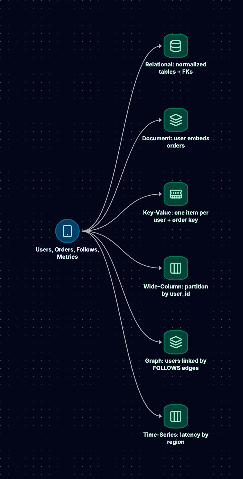
The same domain looks very different in each model. Relational normalizes it into tables, document embeds orders inside the user, key-value designs keys around access patterns, wide-column builds one table per query, graph promotes FOLLOWS and BOUGHT to first-class edges, and time-series keeps only the metrics.
| Dimension | Relational | Document | Key-Value | Wide-Column | Graph | Time-Series |
|---|---|---|---|---|---|---|
| Data model | Tables, rows, foreign keys | JSON/BSON documents | Opaque value or item by key | Partitions of sorted rows | Nodes and relationships | Timestamped points |
| Schema flexibility | Strict, migrations | Flexible per document | Flexible | Fixed columns per table | Flexible properties | Fixed shape, flexible tags |
| Query flexibility | Highest (ad hoc SQL) | High within a collection | Lowest (key and sort key) | Low (designed per query) | High for traversals | High for time ranges |
| Joins | Native and optimized | $lookup, limited | None | None | Traversals replace joins | Yes in TimescaleDB; limited in InfluxDB |
| Transactions | Full multi-row ACID | Single-document; multi-document with cost | Single item; DynamoDB has limited multi-item transactions | Single partition; LWT via Paxos | Full ACID | Mostly append-only |
| Consistency | Strong on primary | Strong on primary by default | Tunable (DynamoDB), primary (Redis) | Tunable per query | Strong on leader | Strong on single node |
| Horizontal write scaling | Hard (manual sharding or distributed SQL) | Built-in sharding | Built-in, near limitless | Built-in, near linear | Limited | Moderate |
| Write throughput | Good, bounded by one primary | High | Very high | Very high | Moderate | Very high for appends |
| Read latency | Low with indexes | Low by key or index | Lowest (sub-ms in memory) | Low within a partition | Low for local traversals | Low for recent windows |
| Operational cost | Moderate; managed options mature | Moderate | Low (managed) to moderate | High (repairs, compaction, tuning) | Moderate | Low to moderate |
| Typical workloads | Orders, payments, inventory, accounts | Catalogs, profiles, CMS | Sessions, caches, carts, high-scale lookups | Messages, events, feeds, IoT at scale | Recommendations, fraud, networks | Metrics, telemetry, monitoring |
Two rows deserve emphasis. Query flexibility and horizontal write scaling pull in opposite directions: the more a database can answer questions you did not plan for, the harder it is to spread its writes across machines. Every type in this table is a different point on that curve.
When to Pick Which
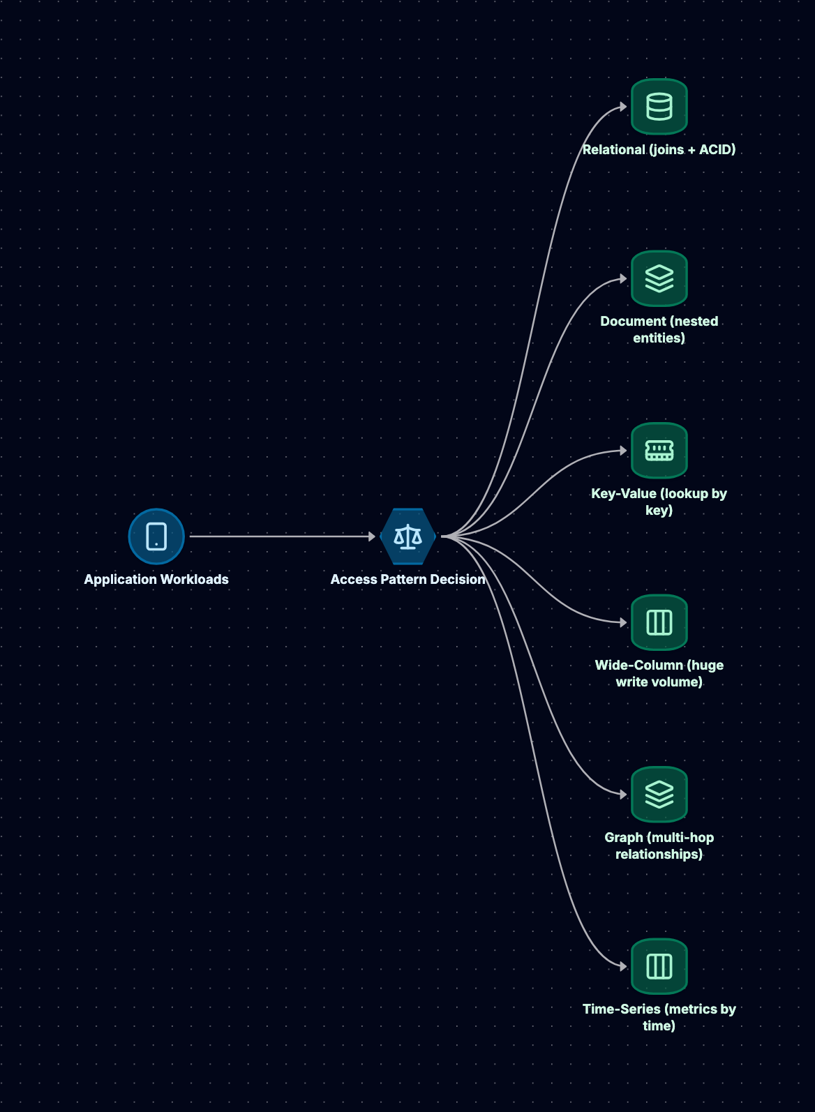
Start from the access patterns, not from the product names. The flowchart below is the order in which I ask the questions.
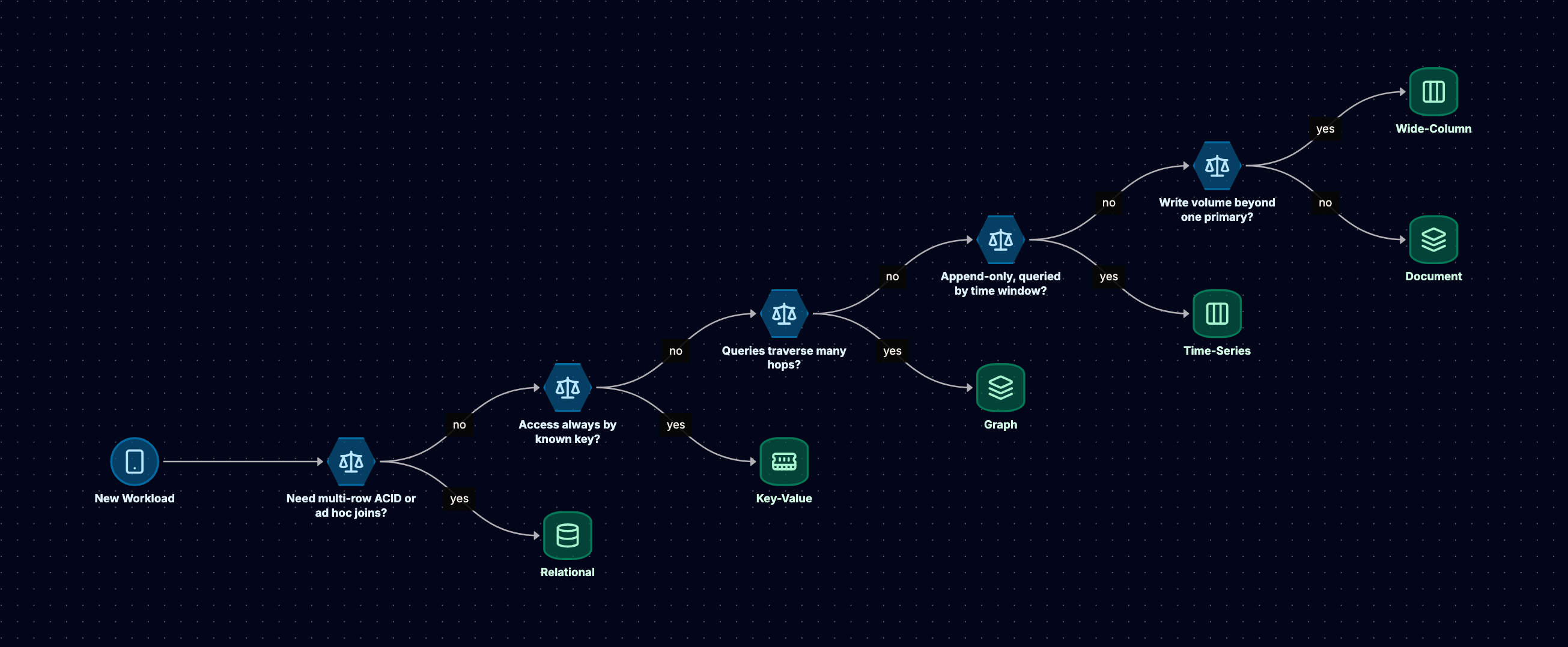
The first question is deliberately relational. If you need multi-row invariants (stock never goes negative, a ledger always balances), you need transactions, and the honest default is PostgreSQL until scale proves otherwise.
Scenario 1: E-commerce Checkout
Requirements: an order, its line items, a stock decrement, and a payment record must commit together or not at all. Reads are by order and by user; finance needs ad hoc reporting.
Choice: PostgreSQL (or Aurora) as the system of record. SELECT ... FOR UPDATE or a conditional UPDATE ... WHERE stock >= 1 enforces the stock invariant, and the transaction makes order creation atomic. Put the shopping cart and sessions in Redis or DynamoDB, because they are keyed, short-lived, and high volume. Ship the product catalog to a search index for browsing.
What I'd say if pushed on scale: shard by user_id or merchant_id so that a checkout stays within one shard, or move to a distributed SQL database (Spanner, CockroachDB, Aurora DSQL) if cross-shard transactions are unavoidable. Do not move money to an eventually consistent store to win a benchmark.
Scenario 2: IoT Telemetry
Requirements: 100,000 devices sending a reading every 10 seconds is 10,000 points per second, around 864 million per day. Queries are "last 24 hours for this device" and "hourly averages by region". Raw data is worth keeping for 30 days, rollups for years.
Choice: TimescaleDB if you also want SQL joins with device metadata in Postgres, or InfluxDB if the team wants a purpose-built metrics engine. Partition by time, segment by device_id, compress after a few days, keep continuous aggregates for the long tail, and drop raw chunks after 30 days.
When it changes: at hundreds of millions of devices or multi-region active-active ingest, Cassandra with a ((device_id, day), ts) key becomes the better fit, with rollups computed by a stream processor.
Scenario 3: Social Feed
Requirements: users follow other users; opening the app shows recent posts from people you follow; reads vastly outnumber writes; celebrity accounts have millions of followers.
Choice: a polyglot design. Users and accounts in PostgreSQL. Posts in Cassandra or DynamoDB, partitioned by author. Precomputed home timelines (lists of post IDs) in Cassandra or Redis, written by fan-out workers, with celebrities handled by pulling their posts at read time instead of pushing to millions of timelines. If the product leans on "people you may know" or multi-hop recommendations, a graph database (or a graph computed offline) serves that one feature.
Polyglot Persistence in Practice
Each scenario above ends with more than one database. That is normal, but every additional store is another system to operate, secure, back up, and keep consistent. The pattern that keeps it manageable:
- One system of record per piece of data. Orders live in PostgreSQL; the copy in the search index or cache is derived and can be rebuilt.
- Propagate changes asynchronously and reliably. Use change data capture (Debezium on the Postgres WAL, DynamoDB Streams, MongoDB change streams) or the transactional outbox pattern: write the business row and an
outboxevent in the same transaction, and let a relay publish the event. Avoid dual writes from application code, where one write succeeds and the other silently fails. - Design for staleness in derived stores. The search index may lag by seconds; the UI should tolerate that, and anything that must be correct reads from the system of record.
- Add a store only for a measured need. "We might need graph queries" is not a reason to run Neo4j. A recursive CTE in PostgreSQL handles two-hop queries on a modest dataset; move when the query plans prove it cannot.
A good default for a new product is PostgreSQL plus Redis. Many teams never need a third database; the ones that do usually know exactly which access pattern forced it.
In the Interview
How to Justify a Choice
Use the same four-step structure every time:
- State the access patterns: "Reads are by user ID and time range; writes are 50,000 per second at peak; we never update a row after writing it."
- State the consistency requirement: "A stale like count is fine; a double-charged card is not."
- Name the type, then the product: "That is an append-only, partition-by-key workload, so wide-column, specifically Cassandra with a time-bucketed partition key."
- Name the cost you are accepting: "We lose ad hoc queries, so analytics goes to a warehouse fed by CDC."
The fourth step is the one most candidates skip, and it is the one interviewers listen for.
Common Traps
- "NoSQL scales, SQL does not." PostgreSQL scales reads with replicas and writes with sharding or distributed SQL. NoSQL stores scale writes more easily because they gave up joins and multi-row transactions, not because of magic. Say the trade, not the slogan.
- Choosing by popularity. "MongoDB because it is flexible" is not a reason. Which query is easier, and which invariant becomes your problem?
- Ignoring the partition key. Saying "DynamoDB" or "Cassandra" without naming the partition key, and checking it for hot spots, is half an answer.
- Forgetting the read path. A write-optimized store with no plan for the main query is a common miss. Write the query first.
- One database for everything, or a database for everything. Both extremes lose points. Justify each store you add.
- Unsourced numbers. Use back-of-envelope math from the stated requirements ("10,000 writes per second, 1 KB each, is about 860 GB per day") rather than quoting benchmarks you cannot defend.
Likely Follow-Up Questions
- "What happens when this partition gets hot?" Add a suffix to spread writes (write sharding), cache hot reads, or change the key so the hot entity spans several partitions.
- "How do you keep the cache or search index consistent?" CDC or an outbox, with idempotent consumers and a rebuild path.
- "Your single Postgres primary is at 80% CPU. Now what?" Profile and index first, add read replicas for read traffic, add connection pooling, then shard by the key that keeps transactions local.
- "Why not just use DynamoDB for the orders too?" You can, with DynamoDB transactions for small multi-item writes, but you trade ad hoc queries and reporting, and you must model every access pattern up front.
- "How would you migrate from one to another?" Dual-read behind a feature flag, backfill with CDC, verify with shadow reads, then cut over writes.
Related reading: Globally Distributed SQL Databases like Spanner and CockroachDB and Designing a Distributed In-Memory Cache like Redis Cluster.