Building Globally Distributed SQL Databases: Architecture and Implementation

Introduction

Building a globally distributed SQL database that maintains ACID guarantees while spanning continents represents one of the most challenging problems in distributed systems. Unlike traditional databases that prioritize either consistency or availability, systems like Google Spanner and CockroachDB achieve strong consistency across geographic regions while maintaining acceptable performance. This architecture enables applications to serve users worldwide with single-digit millisecond latencies for local operations while guaranteeing that every transaction appears to execute in a globally consistent order.

The challenge lies in reconciling fundamental constraints: the speed of light imposes a physical lower bound of approximately 1ms per 100km of network distance, while maintaining consistency requires coordination between nodes. A transaction spanning data centers in Virginia and Singapore faces at least 100-150ms of network round-trip time before any processing begins. Despite these constraints, modern distributed SQL databases achieve 99.999% availability for multi-region configurations while processing millions of queries per second.

This post examines the core architectural components that make globally distributed SQL databases possible. We'll explore how data gets partitioned across thousands of machines, how transactions maintain consistency without sacrificing correctness, how clock synchronization enables ordering of events across continents, how consensus protocols ensure agreement despite failures, and how secondary indexes work when data spans multiple regions. Each section builds on quantifiable design decisions backed by production deployments managing petabyte-scale data.

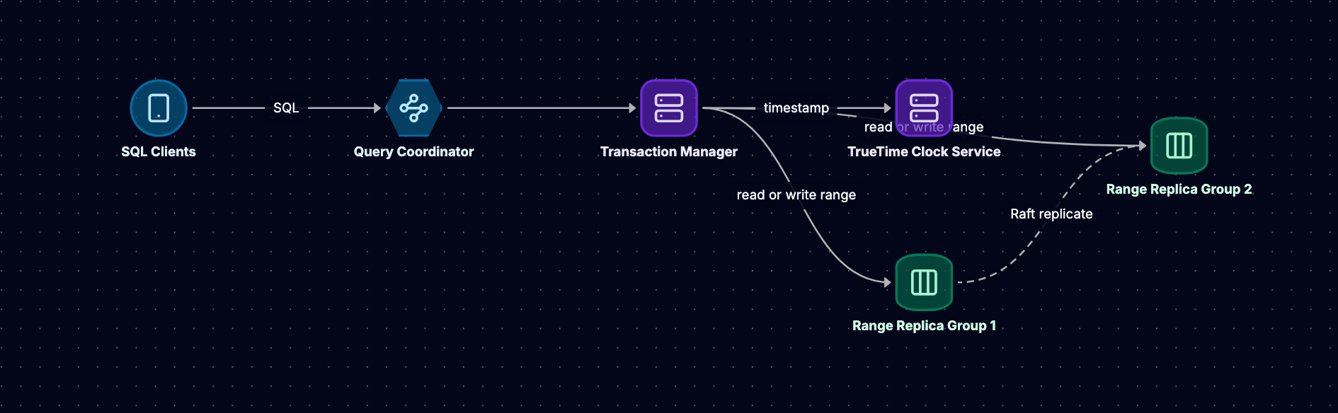
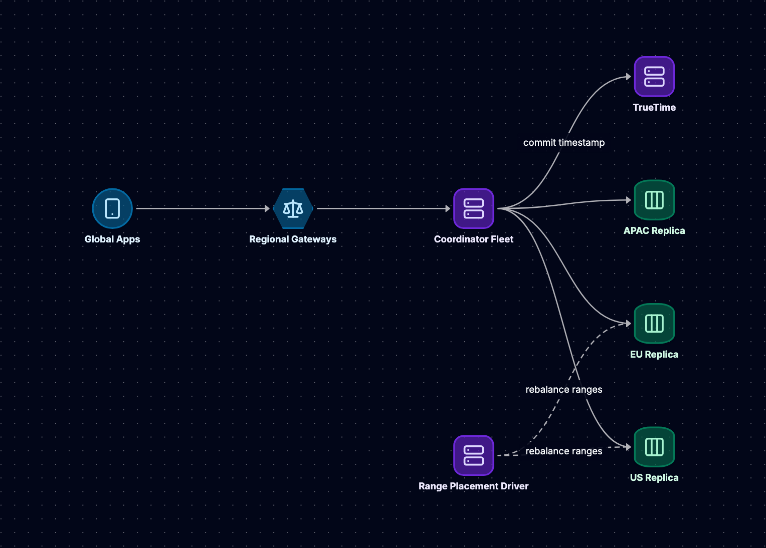
Data Partitioning and Ranges

Distributed SQL databases cannot store all data on a single machine. The solution involves splitting data into ranges, where each range contains a contiguous span of keys typically sized between 64MB and 512MB. When a table grows beyond a single range, the system splits it into multiple ranges that can live on different nodes, enabling horizontal scalability.

Range-Based Partitioning

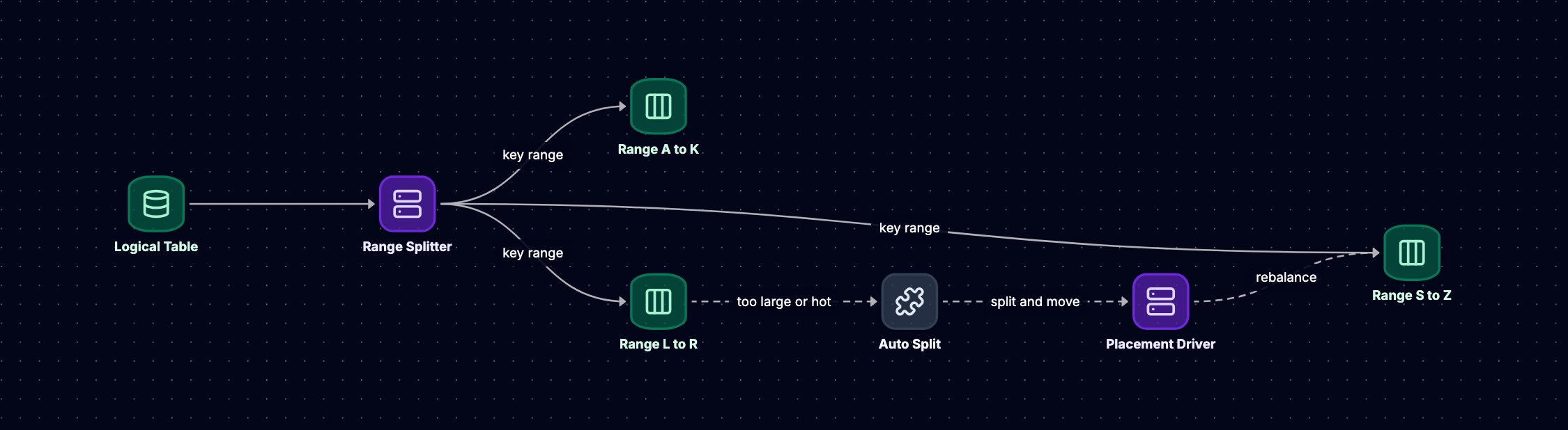
The partitioning strategy uses ordered key-value pairs as the fundamental storage primitive. Consider a table with a primary key: the system orders rows by this key and divides the keyspace into ranges. A range might contain keys from "customer-00000" through "customer-10000", while the next range handles "customer-10001" through "customer-20000". This approach preserves SQL semantics while enabling distribution.

Range boundaries are not static. As data grows, ranges exceeding the size threshold (commonly 512MB) split into two smaller ranges. The system picks a split point, creates two new ranges, and redistributes the data. This split operation happens online without blocking queries. The metadata tracking which ranges exist and where they live gets updated atomically, and subsequent queries route to the correct new ranges.

The benefits of range-based partitioning include efficient range scans (queries like SELECT * FROM orders WHERE order_date BETWEEN '2024-01-01' AND '2024-01-31' touch only relevant ranges) and automatic load balancing (hot ranges can be split and moved to different nodes). The trade-off is that poorly chosen primary keys create hotspots. A table keyed by auto-incrementing integers concentrates all writes on the range containing the highest values, while a UUID-based key distributes writes more evenly.

Range Placement and Replication

Each range exists as multiple replicas across different nodes, with a default replication factor of 3x. One replica serves as the leader (also called leaseholder), handling all writes and strongly consistent reads for that range. Follower replicas receive updates from the leader and can serve stale reads if the application tolerates bounded staleness.

The system distributes replicas across failure domains. For a three-replica range, the database places one replica in each of three different availability zones within a region, or across three different regions for geo-distributed data. This placement strategy ensures that losing an entire zone or region doesn't make data unavailable. The quorum requirement of (N/2 + 1) nodes means a three-replica range tolerates one failure while maintaining write availability.

Replica placement follows explicit constraints defined by administrators. A financial application might specify that European customer data must have all replicas within EU regions for regulatory compliance, while keeping US customer data in North American regions. The system respects these constraints during initial placement and when rebalancing load. Rebalancing typically proceeds at 10-100 GB/hour per node, moving ranges from overloaded nodes to underutilized ones without downtime.

Metadata Management

Tracking which ranges exist and where their replicas live requires a metadata system. This metadata forms a hierarchy: a root range (that never splits) contains pointers to meta ranges, which contain pointers to actual data ranges. Looking up a key requires at most two metadata lookups, and aggressive caching keeps the hot metadata in memory with typical cache hit rates above 99%.

When a range splits, the system updates metadata atomically using a transaction. Clients cache range location information, and when they send a request to the wrong node (because a range moved), they receive a redirect with updated location information. This approach tolerates stale caches while ensuring correctness. The measured cache miss penalty varies by network topology but doesn't fundamentally limit system performance due to high cache hit rates.

Distributed Transactions and Two-Phase Commit

Distributed transactions enable operations spanning multiple ranges (potentially on different nodes across different continents) to execute atomically. A banking application transferring money between accounts needs to debit one account and credit another as a single atomic operation, even when those accounts live in ranges on different continents.

Transaction Execution Model

Each transaction receives a provisional timestamp when it begins. The system tracks all reads (the read set) and all writes (the write set) performed by the transaction. For reads, the system checks that no other transaction has modified the data since the provisional timestamp. For writes, the system buffers changes locally without making them visible to other transactions.

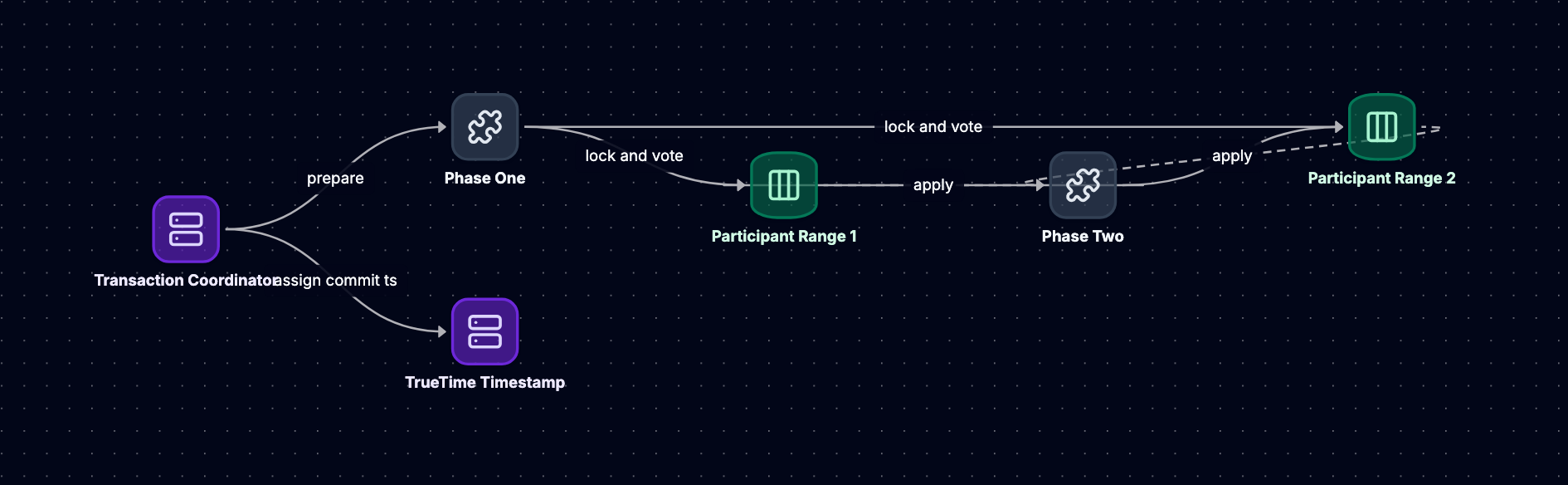
When the application commits, the transaction coordinator (typically the node where the transaction began) initiates a two-phase commit protocol. In the prepare phase, the coordinator sends prepare messages to all nodes participating in the transaction. Each participant checks for conflicts: has another transaction modified data in this transaction's read set, or written to keys in this transaction's write set? If no conflicts exist, the participant votes "yes" and persists a prepare record. If conflicts exist, it votes "no".

The coordinator collects votes from all participants. If every participant voted "yes", the coordinator commits the transaction by persisting a commit record and notifying all participants to apply their buffered writes. If any participant voted "no", the coordinator aborts the transaction. This two-phase protocol ensures atomicity: either all participants commit or all abort, with no partial states visible.

Handling Failures During Commit

The two-phase commit protocol must handle failures at any point. If a participant fails after voting "yes" but before receiving the final commit/abort decision, it remains in an uncertain state. The participant cannot unilaterally commit (other participants might have voted "no") or abort (other participants might have committed). It must wait for the coordinator's decision.

If the coordinator fails after some participants voted "yes", those participants remain blocked until the coordinator recovers. The coordinator persists its state before sending commit/abort decisions, so recovery involves reading this state and completing the protocol. Measured mean time to repair (MTTR) for coordinator failures ranges from 10-60 seconds, during which participants holding locks on data remain blocked.

This blocking behavior represents a fundamental limitation of two-phase commit. If the coordinator fails permanently, participants cannot make progress. Production systems mitigate this through aggressive timeouts and automated failover, but the theoretical possibility of indefinite blocking remains.

Optimizations and Performance

Two-phase commit adds latency: the protocol requires at least two network round-trips (prepare, then commit) between coordinator and participants. For a transaction spanning Virginia and Singapore, this adds 200-400ms of coordination overhead before considering the actual work of reading and writing data.

Several optimizations reduce this cost. Read-only transactions bypass two-phase commit entirely, reading data at a consistent snapshot timestamp without coordination. Single-range transactions (where all reads and writes touch one range) use single-phase commit, as the range leader can commit locally without coordinating with other nodes. Batching multiple small transactions into a single larger transaction amortizes coordination overhead.

Measured transaction throughput varies by workload, but systems demonstrate capability for millions of queries per second across the cluster. Simple transactions within a single region achieve 5-10ms commit latency at the 50th percentile, while cross-region transactions show 50-100ms latency reflecting network distances.

Clock Synchronization and TrueTime

Ordering events in a distributed system requires knowing which events happened before others. In a single-machine database, the system uses a monotonically increasing counter. In a distributed database spanning continents, no single counter exists, and clock skew between machines creates ambiguity about event ordering.

The Clock Skew Problem

Each machine has its own clock, and these clocks drift relative to each other. Standard NTP (Network Time Protocol) synchronization provides accuracy within ±250ms under normal conditions, but this uncertainty creates problems for transaction ordering. If a transaction commits at timestamp 100 on machine A, and another commits at timestamp 105 on machine B, we cannot definitively say which committed first if clock uncertainty exceeds 5ms.

Incorrect ordering violates external consistency (also called linearizability): if transaction T1 completes before transaction T2 begins (as observed by wall-clock time), then T1's timestamp must be less than T2's timestamp. Without bounded clock uncertainty, the system cannot guarantee this property.

Google Spanner's TrueTime

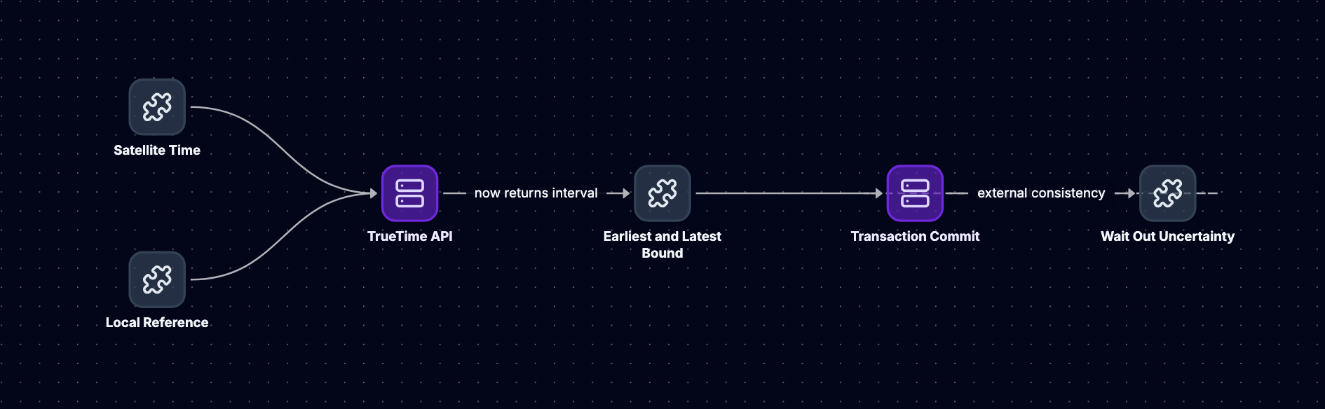
Spanner solves clock uncertainty with TrueTime, an API that exposes clock uncertainty as a first-class concept. Instead of returning a single timestamp, TrueTime returns an interval: [earliest, latest]. The true time lies somewhere within this interval with very high probability. Spanner uses GPS receivers and atomic clocks in each datacenter, achieving uncertainty bounds (epsilon) typically less than 7ms, often between 1-5ms in practice.

The TrueTime API provides three methods: TT.now() returns the current time interval, TT.after(t) returns true if t has definitely passed, and TT.before(t) returns true if t definitely hasn't occurred yet. Transactions use these primitives to ensure correct ordering.

When committing a write transaction, Spanner picks a commit timestamp s within the TrueTime interval. Before returning success to the client, Spanner waits until TT.after(s) returns true. This commit wait ensures that the commit timestamp has definitely passed according to TrueTime. Any transaction starting after the commit wait completes will receive a timestamp greater than s, preserving external consistency.

The commit wait duration equals the TrueTime uncertainty bound, typically less than 7ms. This wait happens in parallel with replication (the system can replicate data to followers while waiting for time to pass), so the added latency is less than the raw uncertainty bound. The trade-off is clear: tighter clock synchronization enables lower latency transactions.

CockroachDB's Hybrid Logical Clocks

CockroachDB uses a different approach: Hybrid Logical Clocks (HLC) that combine physical time from NTP with logical counters. Each timestamp includes a physical component (wall-clock time) and a logical component (a counter that increments when events occur at the same physical time). When nodes communicate, they exchange timestamps and advance their local clocks to ensure causality.

HLC timestamps preserve causality without requiring tight clock synchronization. If event A happens before event B, A's HLC timestamp will be less than B's HLC timestamp. However, HLC depends on NTP synchronization (typically ±250ms) for the physical component, resulting in looser bounds than TrueTime.

CockroachDB implements uncertainty intervals similar to TrueTime. When reading data, a transaction must consider that timestamps on other nodes might be skewed. The system tracks the maximum clock offset observed and uses this to define uncertainty windows. Reads within the uncertainty window may need to be restarted if the system discovers data with ambiguous ordering.

Impact on Transaction Performance

Clock synchronization directly affects transaction latency. Spanner's commit wait adds latency proportional to clock uncertainty. With 7ms uncertainty, write transactions wait up to 7ms before completing. Read-only transactions avoid this wait by using slightly stale snapshots that are guaranteed to be consistent.

CockroachDB's looser clock synchronization affects transaction restarts rather than commit latency. Transactions reading data may encounter uncertainty and need to restart with a higher timestamp. The frequency of restarts depends on workload contention and clock skew. In practice, with properly synchronized NTP, restart rates remain low for most workloads.

Consensus-Based Replication

Replicating data across multiple nodes requires consensus: all replicas must agree on the order of writes. If two clients concurrently write different values to the same key, every replica must apply these writes in the same order to maintain consistency. Consensus protocols solve this problem despite node failures and network partitions.

Raft Consensus Protocol

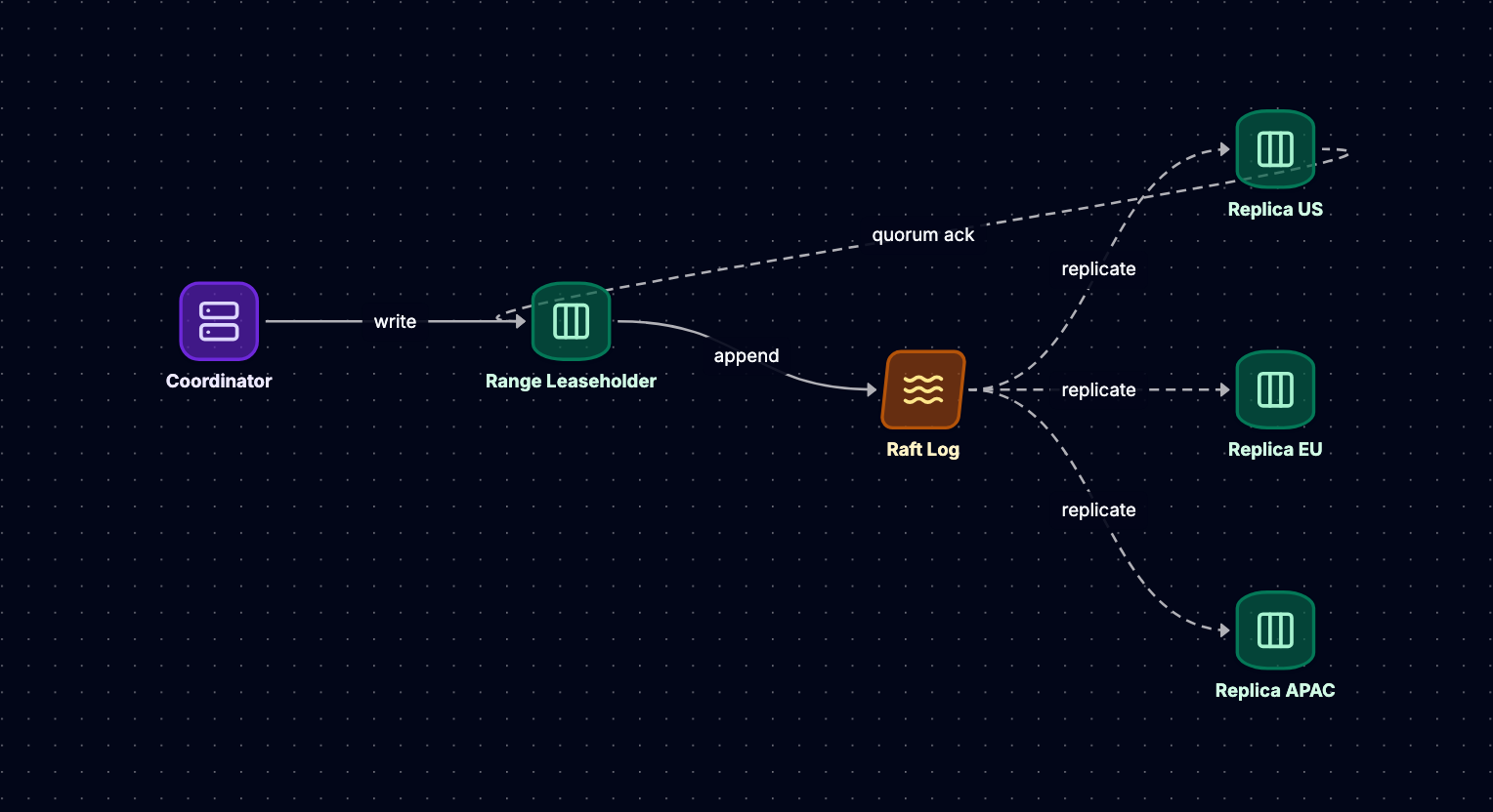
CockroachDB uses Raft, a consensus protocol designed for understandability. In Raft, each range forms a consensus group with one leader and multiple followers. The leader receives all write requests, appends them to its log, and replicates log entries to followers. Once a majority of replicas (quorum) acknowledge the entry, the leader commits it and applies the write to the state machine.

Leader election occurs when the current leader fails or becomes unreachable. Followers start an election timeout (randomized to avoid split votes), and if they don't hear from the leader before timeout, they become candidates and request votes. A candidate receiving votes from a quorum becomes the new leader. Election typically completes within seconds, though this is distinct from the overall MTTR which includes detecting the failure and redirecting traffic.

Raft's quorum requirement means a three-replica group tolerates one failure, and a five-replica group tolerates two failures. The trade-off is that more replicas increase replication overhead: each write must be acknowledged by more nodes before committing. Measured write latency scales with the slowest node in the quorum.

Paxos Variants in Spanner

Spanner uses Paxos, specifically Multi-Paxos optimized for the common case of a stable leader. Like Raft, Paxos ensures that replicas agree on a sequence of values despite failures. The protocol involves proposers (nodes that propose values), acceptors (nodes that vote on proposals), and learners (nodes that learn the chosen value).

Multi-Paxos optimizes the basic Paxos protocol by electing a stable leader that can propose values without the full Paxos protocol for each value. This reduces the number of message round-trips from two to one in the common case. The leader appends entries to its log and replicates them to followers, similar to Raft.

Both Raft and Paxos provide the same safety guarantees: once a value is chosen (committed by a quorum), it will never change. They differ in how they achieve this goal and in their presentation, but both are suitable for building strongly consistent distributed systems.

Replication Lag and Consistency

Synchronous replication (waiting for quorum acknowledgment before committing) ensures that committed data survives failures but adds latency. The leader cannot commit a write until it receives acknowledgments from a quorum of replicas. For replicas in different datacenters, this means waiting for cross-datacenter network round-trips, typically less than 100ms within a region but 50-300ms across regions depending on geographic distance.

The system positions replicas strategically to balance latency and fault tolerance. For data that must survive regional failures, placing replicas across three regions is necessary, accepting the higher write latency. For data that only needs to survive zone failures within a region, placing replicas across three zones provides lower latency (5-10ms) while maintaining fault tolerance.

Follower reads offer an alternative for read-heavy workloads. Instead of reading from the leader (which guarantees the most recent data), clients can read from nearby followers, accepting staleness of 1-10 seconds. This reduces read latency by 50-90% when the nearest follower is geographically closer than the leader. Applications must explicitly opt into stale reads, as the default strong read goes to the leader.

Failure Detection and Recovery

Detecting failures quickly minimizes unavailability. Nodes send periodic heartbeats to each other, and missing heartbeats indicate potential failure. However, distinguishing between a slow node and a failed node is challenging: aggressive timeouts cause false positives (declaring a slow node dead), while conservative timeouts delay failover.

Production systems tune failure detection based on expected network latency and variance. Within a datacenter, heartbeat intervals of 100-500ms enable failure detection within seconds. Across regions, longer intervals (1-5 seconds) reduce false positives from transient network issues.

Once a failure is detected, the consensus protocol elects a new leader. The new leader ensures it has all committed data by communicating with a quorum of replicas. Any in-flight transactions coordinated by the failed node may need to be retried by clients. The measured recovery time from node failure to full operation typically ranges from 10-60 seconds, including detection, election, and client retry.

Global Secondary Indexes

Secondary indexes enable efficient queries on non-primary-key columns. A table of orders keyed by order_id might need an index on customer_id to quickly find all orders for a customer. In a distributed database, maintaining these indexes across ranges and regions adds complexity.

Index Storage and Partitioning

A secondary index is stored as a separate key-value space, where keys are the indexed column values and values are pointers to the primary key. For an index on customer_id, the index stores entries like (customer_id, order_id) pairs. This index gets partitioned into ranges just like the base table, enabling it to scale independently.

Two partitioning strategies exist: local indexes and global indexes. Local indexes partition by the same key as the base table. Each range of the base table has a corresponding index range covering only the rows in that base range. Queries using the index must scatter to all ranges, as data for a given customer_id might exist in any range.

Global indexes partition by the indexed column itself. All entries for a given customer_id live in the same index range, enabling efficient lookups. However, writes become more expensive: inserting a row requires writing to the base table range (determined by the primary key) and the index range (determined by the indexed column), which may live on different nodes across different regions.

Maintaining Index Consistency

Keeping indexes consistent with the base table requires transactional updates. When inserting a row, the system must atomically write both the base table entry and all corresponding index entries. This uses the same distributed transaction mechanism described earlier: the transaction coordinator ensures that either all writes commit or all abort.

For a global index spanning regions, a single row insert might require a distributed transaction across multiple regions. An order inserted in Virginia for a customer indexed in Singapore requires coordination between Virginia (where the order data lives based on order_id) and Singapore (where the index entry lives based on customer_id). This cross-region coordination adds latency, measured at 50-200ms depending on geographic distance.

Index maintenance overhead scales with the number of indexes. Each additional index adds writes during inserts and updates, consuming additional network bandwidth and storage. Production systems balance query performance (more indexes enable faster queries) against write performance (fewer indexes reduce write amplification).

Index-Only Scans and Covering Indexes

A covering index includes not just the indexed column but also other columns frequently queried together. An index on (customer_id, order_date, order_total) enables queries that filter by customer_id and return order_date and order_total without accessing the base table. This avoids the extra lookup to retrieve the full row.

Index-only scans reduce query latency by reading less data. Instead of reading the index to find primary keys, then reading the base table to retrieve rows, the query reads only the index. For queries spanning multiple ranges, this reduces both network traffic and disk I/O. Measured query performance for index-only scans shows 5-50ms for range queries depending on data distribution and result set size.

The trade-off is increased storage: covering indexes duplicate data from the base table into the index. A table with many columns and many covering indexes can consume several times more storage than the base table alone. Compression ratios of 2-5x help mitigate this overhead, but storage costs remain a consideration.

Interleaved Tables and Locality

Some distributed databases support interleaved tables (also called table hierarchies), where child table rows are physically stored adjacent to their parent table rows. Orders for a customer can be stored physically near the customer record, ensuring that queries for a customer and their orders touch only a single range.

Interleaving improves query performance by reducing the number of ranges accessed. A query joining customers and orders can execute entirely within one range if the data is interleaved, avoiding distributed joins across multiple ranges. This reduces latency from tens of milliseconds to single-digit milliseconds for common access patterns.

However, interleaving constrains data distribution. All orders for a customer must live in the same range as the customer, potentially creating hotspots if some customers have many orders. The system cannot split a customer and their orders across multiple ranges, limiting scalability for highly skewed data distributions.

Putting It All Together: A Worked Example

Consider an e-commerce platform serving customers globally. The orders table uses order_id as primary key and has a secondary index on customer_id. Customer data is geo-partitioned: European customers have data in EU regions, US customers in US regions.

When a European customer places an order, the application begins a transaction. The transaction reads the customer's shipping address (from a range in an EU region) and reads product inventory (from a range potentially in a different region). It then writes a new order record (to a range determined by order_id) and updates the inventory count.

If the order_id hashes to a range in a US region while the customer_id index range lives in an EU region, the transaction spans continents. The coordinator (likely in the EU region where the transaction began) executes two-phase commit. In the prepare phase, it sends prepare messages to participants in both the US region (for the order record) and the EU region (for the index entry). Network round-trip time between these regions is 100-150ms.

Each participant checks for conflicts using the transaction's timestamp. The US participant verifies no other transaction modified the order_id key. The EU participant verifies no other transaction modified the customer_id index entry. Both vote "yes" and persist prepare records. The coordinator receives both votes, persists a commit record, and sends commit messages to participants.

Before responding to the client, the coordinator waits for the commit timestamp to pass (in Spanner) or ensures no uncertainty windows overlap (in CockroachDB). The total latency includes network round-trips (100-150ms each way), prepare/commit processing (5-10ms per phase), and commit wait (up to 7ms for Spanner). The measured end-to-end latency for this cross-region transaction falls in the 200-300ms range, dominated by network latency.

For read-heavy queries like "show me all orders for this customer", the application uses the secondary index on customer_id. The query routes to the index range, which returns order_id values for that customer. If the query needs full order details, it then fetches rows from the base table. With proper index design (covering index including order date and total), the query completes in 10-50ms for typical result set sizes.

Operational Considerations

Running a globally distributed SQL database in production requires attention to several operational aspects beyond the core architecture.

Resource Requirements and Capacity Planning

Each node requires sufficient CPU, memory, and disk I/O to handle its share of the workload. Measured CPU overhead for consensus and coordination ranges from 10-30% of total CPU usage. Memory requirements start at 2-4 GB per node minimum, with 16-64 GB recommended for production workloads to cache hot data and metadata.

Disk I/O requirements depend on workload characteristics. Write-heavy workloads generate 1000-10000 IOPS per node, while read-heavy workloads with good cache hit rates generate less disk I/O. The storage engine (commonly RocksDB with LSM-tree structure) exhibits write amplification of 10-30x depending on compaction patterns and data size.

Network bandwidth between regions becomes a bottleneck for cross-region transactions. Replicating data across continents requires sustained bandwidth, with production deployments provisioning 100Mbps to 10Gbps between regions depending on workload. Monitoring network saturation prevents performance degradation.

Monitoring and Observability

Production systems expose hundreds of metrics for monitoring cluster health. Key metrics include transaction latency (p50, p99, p999), replication lag (typically less than 100ms for synchronous replication), range count and distribution, and resource utilization per node.

Distributed tracing helps diagnose slow queries. A query touching multiple ranges across regions generates trace spans showing time spent in each phase: query planning, range routing, network communication, consensus coordination, and result aggregation. This visibility enables identifying bottlenecks.

Alerting on anomalies prevents outages. Sustained increases in transaction latency might indicate network issues or overloaded nodes. Replication lag spikes suggest follower nodes falling behind. Proactive monitoring and automated remediation (like rebalancing ranges away from overloaded nodes) maintain system health.

Backup and Disaster Recovery

Despite synchronous replication providing durability, backups protect against logical corruption (application bugs that write incorrect data) and catastrophic failures. The system supports consistent snapshots: point-in-time copies of all data that represent a transactionally consistent state.

Snapshot frequency ranges from minutes to hours depending on recovery point objective (RPO) requirements. Near-zero RPO is achievable with synchronous replication alone, as committed data exists on multiple replicas. Snapshots provide additional protection with configurable retention periods.

Recovery time objective (RTO) for full cluster recovery from backups ranges from minutes to hours depending on data size. Restoring petabyte-scale databases takes longer than gigabyte-scale databases. Incremental backups and parallel restore processes reduce recovery time.

Schema Changes and Migrations

Altering table schemas (adding columns, creating indexes) in a distributed database requires coordination across all nodes. The system must ensure that all nodes agree on the schema version before applying changes. Online schema changes allow queries to continue during the migration, but with added complexity.

Creating a new index on a large table triggers a distributed backfill: the system scans all existing rows and